Principal Components Analysis
Contents
Principal Components Analysis#
Some facts#
This is the most popular unsupervised procedure ever.
Invented by Karl Pearson (1901).
Developed by Harold Hotelling (1933). \(\leftarrow\) Stanford pride!
What does it do? It provides a way to visualize high dimensional data, summarizing the most important information.
What is PCA good for?#
All pairs scatter |
Biplot for first 2 principal components |
|---|---|

|

|
What is the first principal component?#
It is the line which passes the closest to a cloud of samples, in terms of squared Euclidean distance.

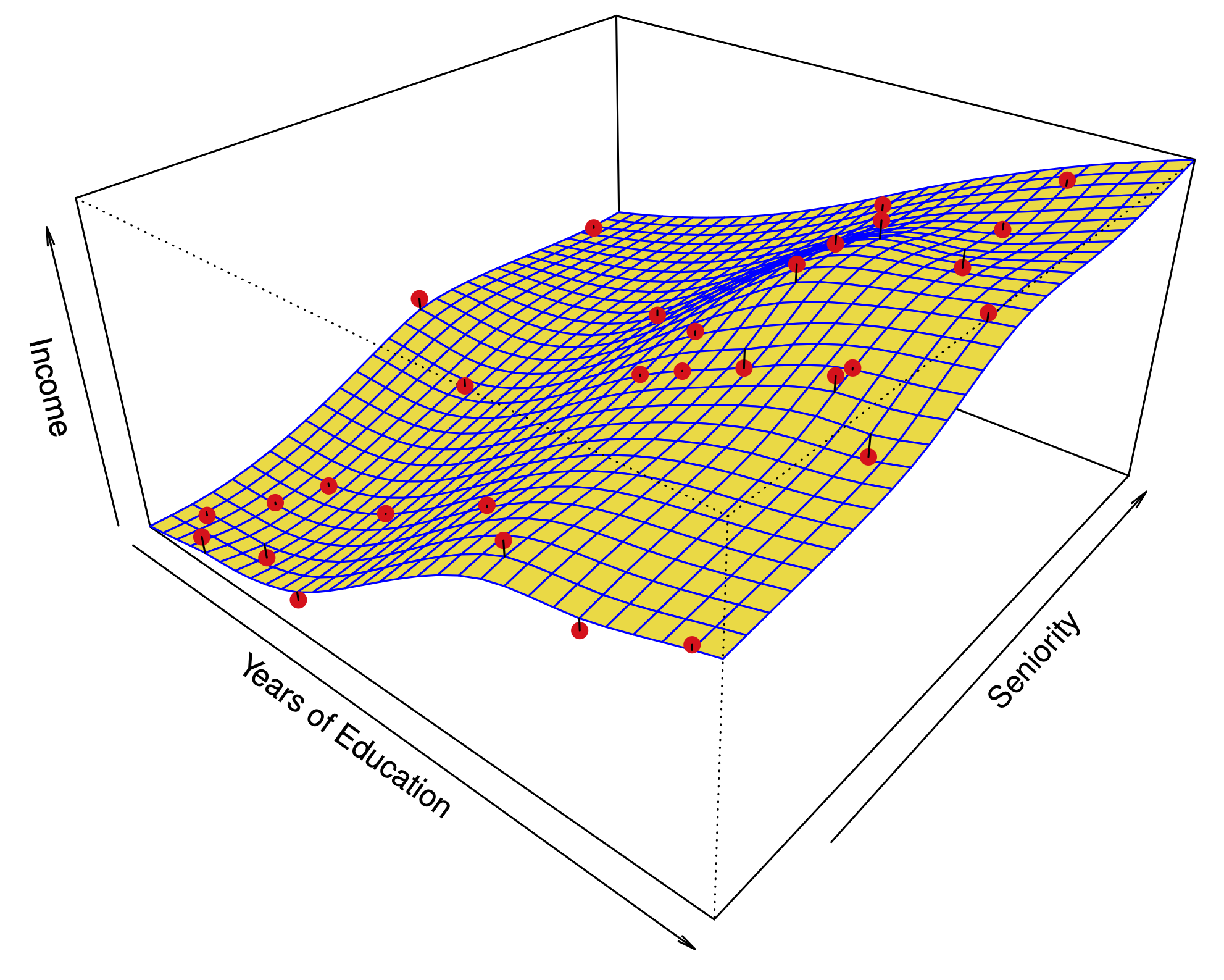
What does this look like with 3 variables?#
The first two principal components span a plane which is closest to the data.
Fig 10.2a |
Fig 10.2b |
|---|---|

|

|
A second interpretation#
The projection onto the first principal component is the one with the highest variance.

How do we say this in math?#
Let \(\mathbf{X}\) be a data matrix with \(n\) samples, and \(p\) variables.
From each variable, we subtract the mean of the column; i.e. we center the variables.
To find the first principal component \(\phi_1 = (\phi_{11},\dots,\phi_{p1})\), we solve the following optimization
The quantity
Summing the square of the entries of \(Z\) computes the variance of the \(n\) samples projected onto \(\phi_1\). (This is a variance because we have centered the columns.)
Having found the maximizer \(\hat{\phi}_1\), the the first principal component score is
Second principal component#
To find the second principal component \(\phi_2 = (\phi_{12},\dots,\phi_{p2})\), we solve the following optimization
The second constraint \(\hat{\phi}_1'\phi_2=0\) forces first and second principal components to be orthogonal.
Having found the optimal \(\hat{\phi}_2\), the second principal component score is
It turns out that the constraint \(\hat{\phi}_1'\phi_2=0\) implies that the scores \(Z_1=(z_{11},\dots,z_{n1})\) and \(Z_2=(z_{12},\dots,z_{n2})\) are uncorrelated.
Solving the optimization#
This optimization is fundamental in linear algebra. It is satisfied by either:
The singular value decomposition (SVD) of (the centered) \(\mathbf{X}\): $\(\mathbf{X} = \mathbf{U\Sigma\Phi}^T\)\( where the \)i\(th column of \)\mathbf{\Phi}\( is the \)i\(th principal component \)\hat{\phi}i\(, and the \)i\(th column of \)\mathbf{U\Sigma}\( is the \)i\(th vector of scores \)(z{1i},\dots,z_{ni})$.
The eigendecomposition of \(\mathbf{X}^T\mathbf{X}\):
Biplot#
Scaling the variables#
Most of the time, we don’t care about the absolute numerical value of a variable.
Typically, we care about the value relative to the spread observed in the sample.
Before PCA, in addition to centering each variable, we also typically multiply it times a constant to make its variance equal to 1.
Example: scaled vs. unscaled PCA#

In special cases, we have variables measured in the same unit; e.g. gene expression levels for different genes.
In such case, we care about the absolute value of the variables and we can perform PCA without scaling.
How many principal components are enough?#
We said 2 principal components capture most of the relevant information. But how can we tell?
The proportion of variance explained#
We can think of the top principal components as directions in space in which the data vary the most.
The \(i\)th score vector \((z_{1i},\dots,z_{ni})\) can be interpreted as a new variable. The variance of this variable decreases as we take \(i\) from 1 to \(p\).
The total variance of the score vectors is the same as the total variance of the original variables:
We can quantify how much of the variance is captured by the first \(m\) principal components/score variables.
Scree plot#

The variance of the \(m\)th score variable is:
The scree plot plots these variances: we see that the top 2 explain almost 90% of the total variance.