Linear Discriminant Analysis (LDA)
Contents
Linear Discriminant Analysis (LDA)#
Strategy: Instead of estimating \(P(Y\mid X)\) directly, we could estimate:
\(\hat P(X \mid Y)\): Given the response, what is the distribution of the inputs.
\(\hat P(Y)\): How likely are each of the categories.
Then, we use Bayes rule to obtain the estimate:
LDA: multivariate normal with equal covariance#
LDA is the special case of the above strategy when \(P(X \mid Y=k) = N(\mu_k, \mathbf\Sigma)\).
That is, within each class the features have multivariate normal distribution with center depending on the class and common covariance \(\mathbf\Sigma\).
The probabilities \(P(Y=k)\) are estimated by the fraction of training samples of class \(k\).
Decision boundaries#
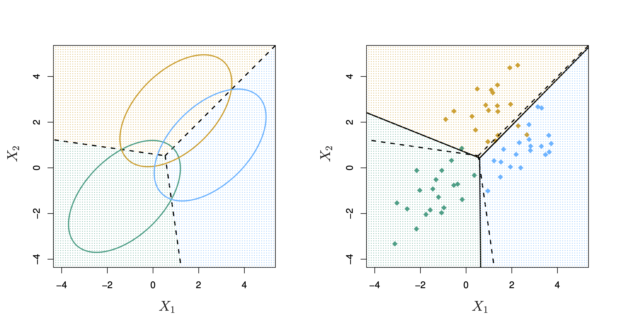
Fig. 17 Density contours and decision boundaries for LDA with three classes.#
LDA has (piecewise) linear decision boundaries#
Suppose that:
We know \(P(Y=k) = \pi_k\) exactly.
\(P(X=x | Y=k)\) is Mutivariate Normal with density:
Above: \(\mu_k:\) Mean of the inputs for category \(k\) and \(\mathbf\Sigma:\) covariance matrix (common to all categories)
Then, what is the Bayes classifier?
By Bayes rule, the probability of category \(k\), given the input \(x\) is:
The denominator does not depend on the response \(k\), so we can write it as a constant:
Now, expanding \(f_k(x)\):
Let’s absorb everything that does not depend on \(k\) into a constant \(C'\):
Take the logarithm of both sides: $\(\log P(Y=k \mid X=x) = \color{Red}{\log C'} + \color{blue}{\log \pi_k - \frac{1}{2}(x-\mu_k)^T \mathbf{\Sigma}^{-1}(x-\mu_k)}.\)$
This is the same for every category, \(k\).
We want to find the maximum of this expression over \(k\).
Goal is to maximize the following over \(k\): $\( \begin{aligned} &\log \pi_k - \frac{1}{2}(x-\mu_k)^T \mathbf{\Sigma}^{-1}(x-\mu_k).\\ =&\log \pi_k - \frac{1}{2}\left[x^T \mathbf{\Sigma}^{-1}x + \mu_k^T \mathbf{\Sigma}^{-1}\mu_k\right] + x^T \mathbf{\Sigma}^{-1}\mu_k \\ =& C'' + \log \pi_k - \frac{1}{2}\mu_k^T \mathbf{\Sigma}^{-1}\mu_k + x^T \mathbf{\Sigma}^{-1}\mu_k \end{aligned} \)$
We define the objectives (called discriminant functions): $\(\delta_k(x) = \log \pi_k - \frac{1}{2}\mu_k^T \mathbf{\Sigma}^{-1}\mu_k + x^T \mathbf{\Sigma}^{-1}\mu_k\)\( At an input \)x\(, we predict the response with the highest \)\delta_k(x)$.
Decision boundaries#
What are the decision boundaries? It is the set of points \(x\) in which 2 classes do just as well (i.e. the discriminant functions of the two classes agree at \(x\)):
This is a linear equation in \(x\).
Decision boundaries revisited#
Fig. 18 Density contours and decision boundaries for LDA with three classes.#
Estimating \(\pi_k\)#
In English: the fraction of training samples of class \(k\).
Estimating the parameters of \(f_k(x)\)#
Estimate the center of each class \(\mu_k\):#
Estimate the common covariance matrix \(\mathbf{\Sigma}\):
One predictor (\(p=1\)):
Many predictors (\(p>1\)): Compute the vectors of deviations \((x_1 -\hat \mu_{y_1}),(x_2 -\hat \mu_{y_2}),\dots,(x_n -\hat \mu_{y_n})\) and use an unbiased estimate of its covariance matrix, \(\mathbf\Sigma\).
Final decision rule#
For an input \(x\), predict the class with the largest:
The decision boundaries are defined by \(\left\{x: \delta_k(x) = \delta_{\ell}(x) \right\}, 1 \leq j,\ell \leq K\).