Generalized Additive Models (GAMs)
Contents
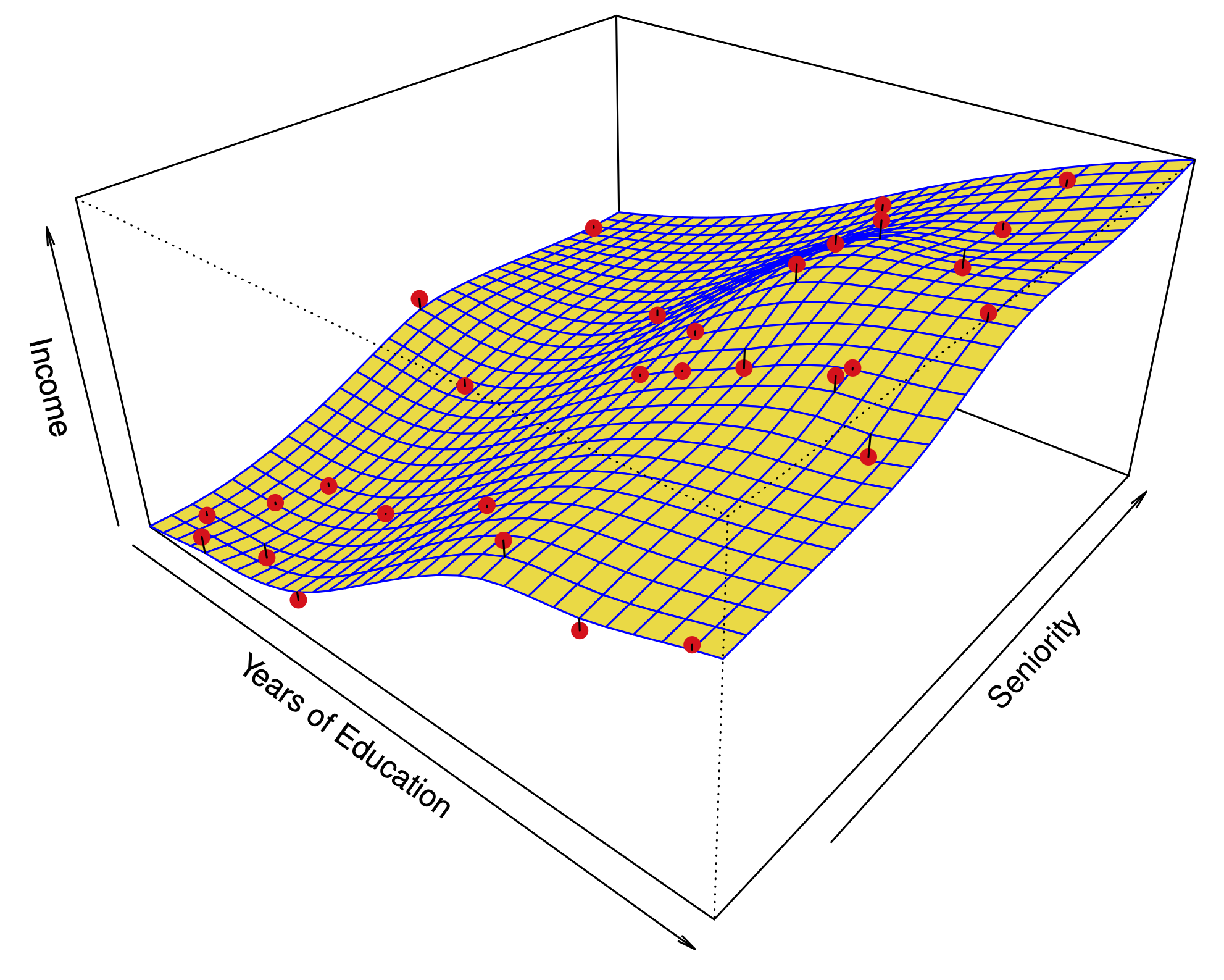
Generalized Additive Models (GAMs)#
Extension of non-linear models to multiple predictors:
The functions \(f_1,\dots,f_p\) can be polynomials, natural splines, smoothing splines, local regressions…
Fitting a GAM#
If the functions \(f_1\) have a basis representation, we can simply use least squares:
Natural cubic splines
Polynomials
Step functions
Backfitting#
Keep \(\beta_0,f_2,\dots,f_p\) fixed, and fit \(f_1\) using the partial residuals as response: $\(y_i - \beta_0 - f_2( x_{i2}) -\dots - f_p( x_{ip}),\)$
Keep \(\beta_0,f_1,f_3,\dots,f_p\) fixed, and fit \(f_2\) using the partial residuals as response: $\(y_i - \beta_0 - f_1( x_{i1}) - f_3( x_{i3}) -\dots - f_p( x_{ip}),\)$
…
Iterate
This works for smoothing splines and local regression.
For smoothing splines this is a descent method, descending on convex loss …
Also works for linear regression…#
Initialize \(\hat{\beta}^{(0)} = 0\) and, (say).
Given \(\hat{\beta}^{(T-1)}\), choose a coordinate \(0 \leq k(T) \leq p\) and find $\( \begin{aligned} \hat{\alpha}(T) &= \text{argmin}_{\alpha} \sum_{i=1}^n\left(Y_i - \hat{\beta}^{(T-1)}_0 - \sum_{j:j \neq k(T)} X_{ij} \hat{\beta}^{(T-1)}_j - \alpha X_{ik(T)}\right)^2 \\ &= \frac{\sum_{i=1}^n X_{ik(T)}\left(Y_i - \hat{\beta}^{(T-1)}_0 - \sum_{j: j \neq k(T)} X_{ij} \hat{\beta}^{(T-1)}_j\right)} {\sum_{i=1}^n X_{ik(T)}^2} \end{aligned} \)$
Set \(\hat{\beta}^{(T)}=\hat{\beta}^{(T-1)}\) except \(k(T)\) entry which we set to \(\hat{\alpha}(T)\).
Iterate
Backfitting: coordinate descent and LASSO#
Initialize \(\hat{\beta}^{(0)} = 0\) and, (say).
Given \(\hat{\beta}^{(T-1)}\), choose a coordinate \(0 \leq k(T) \leq p\) and find $\( \begin{aligned} \hat{\alpha}_{\lambda}(T) &= \text{argmin}_{\alpha} \sum_{i=1}^n\left(r^{(T-1)}_{ik(T)} - \alpha X_{ik(T)}\right)^2 \\ & \qquad + \lambda \sum_{j: j \neq k(T)} |\hat{\beta}^{(T-1)}_j| + \lambda |\alpha| \end{aligned} \)\( with \)r^{(T-1)}_j\( the \)j\(-th partial residual at iteration \)T\( \)\( r^{(T-1)}_j = Y - \hat{\beta}^{(T-1)}_0 - \sum_{l:l \neq j} X_l \hat{\beta}^{(T-1)}_l. \)\( Solution is a simple soft-thresholded version of previous \)\hat{\alpha}(T)$ – Very fast! Used in
glmnetSet \(\hat{\beta}^{(T)}=\hat{\beta}^{(T-1)}\) except \(k(T)\) entry which we set to \(\hat{\alpha}_{\lambda}(T)\).
Iterate…
Backfitting with basis functions#
Initialize \(\hat{\beta}^{(0)} = 0\) and, (say).
Given \(\hat{\beta}^{(T-1)}\), choose a coordinate \(0 \leq k(T) \leq p\) and find $\( \begin{aligned} \hat{\alpha}(T) &= \text{argmin}_{\alpha \in \mathbb{R}^{n_{k(T)}}} \\ & \qquad \sum_{i=1}^n\biggl(Y_i - \hat{\beta}^{(T-1)}_0 - \sum_{j:j \neq k(T)} \sum_{l=1}^{n_j} f_{lj}(X_{ij}) \hat{\beta}^{(T-1)}_{lj} \\ & \qquad \quad - \sum_{l=1}^{n_{k(T)}} \alpha_{l} f_{lk(T)}(X_{ik(T)})\biggr)^2 \end{aligned} \)\( 3.Set \)\hat{\beta}^{(T)}=\hat{\beta}^{(T-1)}\( except \)k(T)\( entries which we set to \)\hat{\alpha}(T)$. (This is blockwise coordinate descent!)
Iterate…
Properties#
GAMs are a step from linear regression toward a fully nonparametric method.
The only constraint is additivity. This can be partially addressed by adding key interaction variables \(X_iX_j\) (or tensor product of basis functions – e.g. polynomials of two variables).
We can report degrees of freedom for many non-linear functions.
As in linear regression, we can examine the significance of each of the variables.
Example: Regression for Wage#

year: natural spline with df=4.age: natural spline with df=5.education: factor.
Example: Regression for Wage#

year: smoothing spline with df=4.age: smoothing spline with df=5.education: step function
Classification#
We can model the log-odds in a classification problem using a GAM:
Again fit by backfitting …
Backfitting with logistic loss#
Initialize \(\hat{\beta}^{(0)} = 0\) and, (say).
Given \(\hat{\beta}^{(T-1)}\), choose a coordinate \(0 \leq k(T) \leq p\) with \(\ell\) logistic loss, find $\( \begin{aligned} \hat{\alpha}(T) &= \text{argmin}_{\alpha \in \mathbb{R}^{n_{k(T)}}} \\ & \qquad \sum_{i=1}^n \ell\biggl(Y_i, \hat{\beta}^{(T-1)}_0 + \sum_{j:j \neq k(T)} \sum_{l=1}^{n_j} f_{lj}(X_{ij}) \hat{\beta}^{(T-1)}_{lj} \\ & \qquad \quad + \sum_{l=1}^{n_{k(T)}} \alpha_{l} f_{lk(T)}(X_{ik(T)}) \biggr) \end{aligned} \)$
Set \(\hat{\beta}^{(T)}=\hat{\beta}^{(T-1)}\) except \(k(T)\) entries which we set to \(\hat{\alpha}(T)\).
Works for losses that have a linear predictor.
For GAMs, the linear predictor is $\( \beta_0 + f_1(X_1) + \dots + f_p(X_p) \)$
Example: Classification for Wage>250#

year: linearage: smoothing spline with df=5education: step function
Example: Classification for Wage>250#

Same model excluding cases
education == "<HS"