Simple linear regression
Contents
Simple linear regression#
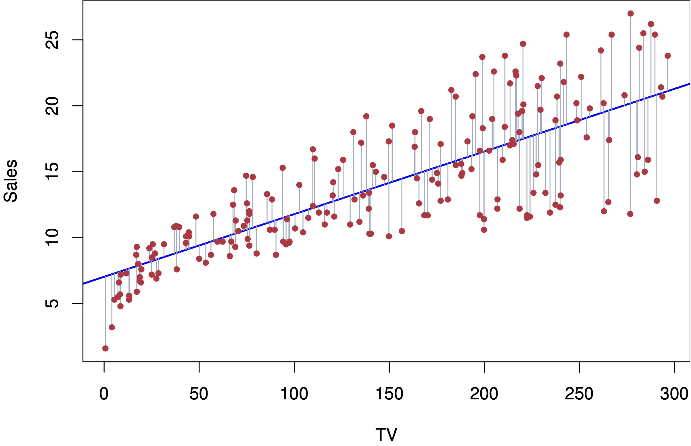
Fig. 9 Simple linear regression#
Model#
Errors: \(\varepsilon_i \sim N(0,\sigma^2)\quad \text{i.i.d.}\)
Fit: the estimates \(\hat\beta_0\) and \(\hat\beta_1\) are chosen to minimize the (training) residual sum of squares (RSS):
Sample code: advertising data#
library(ISLR)
Advertising = read.csv("https://www.statlearning.com/s/Advertising.csv", header=TRUE, row.names=1)
M.sales = lm(sales ~ TV, data=Advertising)
M.sales
Estimates \(\hat\beta_0\) and \(\hat\beta_1\)#
A little calculus shows that the minimizers of the RSS are:
Assessing the accuracy of \(\hat \beta_0\) and \(\hat\beta_1\)#

Fig. 10 How variable is the regression line?#
Based on our model#
The Standard Errors for the parameters are:
95% confidence intervals:
Hypothesis test#
Null hypothesis \(H_0\): There is no relationship between \(X\) and \(Y\).
Alternative hypothesis \(H_a\): There is some relationship between \(X\) and \(Y\).
Based on our model: this translates to
\(H_0\): \(\beta_1=0\).
\(H_a\): \(\beta_1\neq 0\).
Test statistic:
Under the null hypothesis, this has a \(t\)-distribution with \(n-2\) degrees of freedom.
Sample output: advertising data#
summary(M.sales)
confint(M.sales)
Interpreting the hypothesis test#
If we reject the null hypothesis, can we assume there is an exact linear relationship?
No. A quadratic relationship may be a better fit, for example. This test assumes the simple linear regression model is correct which precludes a quadratic relationship.
If we don’t reject the null hypothesis, can we assume there is no relationship between \(X\) and \(Y\)?
No. This test is based on the model we posited above and is only powerful against certain monotone alternatives. There could be more complex non-linear relationships.