Supervised learning
Contents
Supervised learning#
Setup#
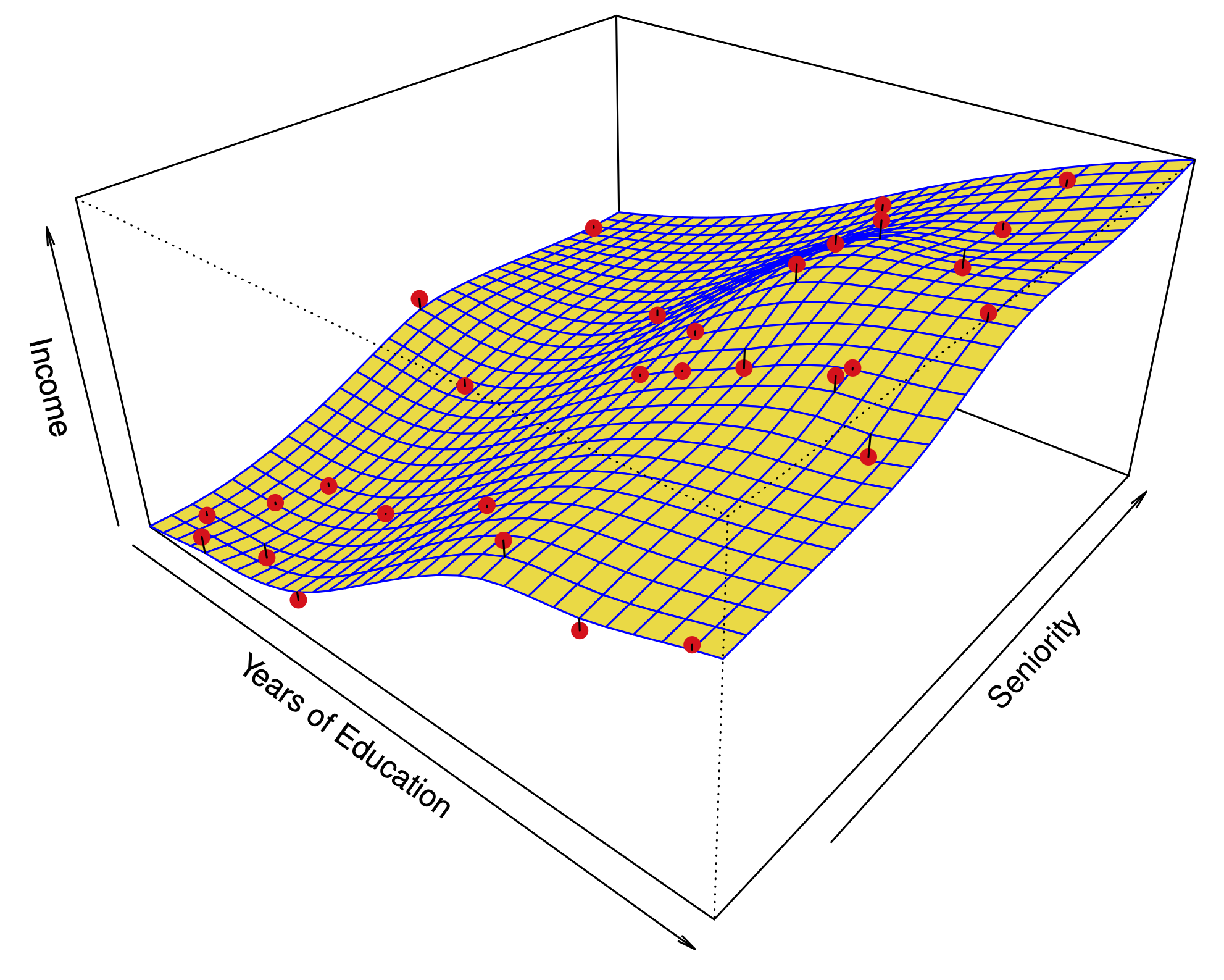
In supervised learning, there are input variables, and output variables:

Fig. 3 Typical regression problem#
Classification problems#
In supervised learning, there are input variables, and output variables:

Fig. 4 Typical classification problem#
Goals of supervised learning#
In supervised learning, there are input variables, and output variables:
If \(X\) is the vector of inputs for a particular sample. The output variable for regression is modeled by:
Our goal is to learn the function \(f\), using a set of training samples \((x_1,y_1)\dots(x_n,y_n)\)
Regression model#
Motivations#
Motivation |
Example |
|---|---|
Prediction: Useful when the input variable is readily available, but the output variable is not. |
Predict stock prices next month using data from last year. |
Inference: A model for \(f\) can help us understand the structure of the data: which variables influence the output, and which don’t? What is the relationship between each variable and the output, e.g. linear, non-linear? |
What is the influence of genetic variations on the incidence of heart disease? |
Parametric and nonparametric methods#
There are (broadly) two kinds of supervised learning method:
Parametric methods: We assume that \(f\) takes a specific form. For example, a linear form:
with parameters \(\beta_1,\dots,\beta_p\). Using the training data, we try to fit the parameters.
Non-parametric methods: We don’t make any assumptions on the form of \(f\), but we restrict how wiggly or rough the function can be.
Parametric vs. nonparametric prediction#
Parametric |
Non-parametric |
|---|---|

|

|
Parametric methods have a limit of fit quality. Non-parametric methods can keep improving as we add more data to fit.
Parametric methods are often simpler to interpret.
Prediction error#
Our goal in supervised learning is to minimize the prediction error
For regression models, this is typically the Mean Squared Error (MSE). Let \((x_0, y_0)\) denote a new sample from the population:
Unfortunately, this quantity cannot be computed, because we don’t know the joint distribution of \((x_0,y_0)\).
We can compute a sample average using the training data; this is known as the training MSE:
\(MSE_{\text{training}}\) can be used to learn \(\hat{f}\)
Key quantities#
Term |
Quantity |
|---|---|
Training data |
\((x_1,y_1),(x_2,y_2)\dots (x_n,y_n)\) |
Predicted function |
\(\hat f\), a function of (i.e. learned on) training data |
Future data |
\((x_0,y_0)\) having some distribution (usually related to distribution of training data) |
Prediction error (MSE) |
\(MSE(\hat f) = E(y_0 - \hat f(x_0))^2.\) |
Test vs. training error#
The main challenge of statistical learning is that a low training MSE does not imply a low MSE.
If we have test data \(\{(x'_i,y'_i);i=1,\dots,m\}\) which were not used to fit the model, a better measure of quality for \(\hat f\) is the test MSE:

Fig. 5 Prediction error vs. flexibility#
The circles are simulated data from the black curve \(f\) by adding Gaussian noise. In this artificial example, we know what \(f\) is.
Three estimates \(\hat f\) are shown: Linear regression, Splines (very smooth), Splines (quite rough).
Red line: Test MSE, Gray line: Training MSE.

Fig. 6 Prediction error vs. flexibility#
The function \(f\) is now almost linear.

Fig. 7 Prediction error vs. flexibility#
When the noise \(\varepsilon\) has small variance relative to \(f\), the third method does well.
The bias variance decomposition#
Let \(x_0\) be a fixed test point, \(y_0 = f(x_0) + \varepsilon_0\), and \(\hat f\) be estimated from \(n\) training samples \((x_1,y_1)\dots(x_n,y_n)\).
Let \(E\) denote the expectation over \(y_0\) and the training outputs \((y_1,\dots,y_n)\). Then, the Mean Squared Error at \(x_0\) can be decomposed:
Term |
Notation |
Description |
|---|---|---|
Variance |
\(\text{Var}(\hat f(x_0))\) |
The variance of the estimate of \(Y\): \(E[\hat f(x_0) - E(\hat f(x_0))]^2\) |
Bias (squared) |
\([\text{Bias}(\hat f(x_0))]^2\) |
This measures how much the estimate of \(\hat f\) at \(x_0\) changes when we sample and average over new training data. |
Irreducible error |
\(\text{Var}(\varepsilon_0)\) |
This is how much of the response is not predictable by any method. |
Each fitting method has its own variance and bias. No method can improve on irreducible error.
A good method has small variance + squared bias.
Simulation example#
Sample #1 |
Sample #2 |
Sample #3 |
Sample #4 |
|---|---|---|---|

|

|

|

|
All fits |
Bias |
|---|---|

|

|
Implications of bias variance decomposition#
The MSE is always positive.
Each element on the right hand side is always positive.
Therefore, typically when we decrease the bias beyond some point, we increase the variance, and vice-versa.
More flexibility \(\iff\) Higher variance \(\iff\) Lower bias.

Squiggly \(f\), high noise
Linear \(f\), high noise
Squiggly \(f\), low noise
Classification problems#
In a classification setting, the output takes values in a discrete set.
For example, if we are predicting the brand of a car based on a number of variables, the function \(f\) takes values in the set \(\{\text{Ford, Toyota, Mercedes-Benz}, \dots\}\).
Model is no longer
We use slightly different notation:
For classification we are interested in learning \(P(Y\mid X)\).
Connection between the classification and regression: both try to learn \(E(Y\mid X)\) but the type of \(Y\) is different.
Loss function for classification#
There are many ways to measure the error of a classification prediction. One of the most common is the 0-1 loss:
Like the MSE, this quantity can be estimated from training or test data by taking a sample average:
For training, we usually use smoother proxies of 0-1 loss – easier to minimize.
While no bias-variance decomposition, test error curves look similar to regression.
Bayes classifier#

Fig. 8 Bayes decision boundary#
The Bayes classifier assigns:
It can be shown that this is the best classifier under the 0-1 loss.
In practice, we never know the joint probability \(P\). However, we may assume that it exists.
Many classification methods approximate \(P(Y=j \mid X=x_i)\) with \(\hat{P}(Y=j \mid X=x_i)\) and predict using this approximate Bayes classifier.