Gaussian Model

In week 8, we turned to our final topic in this little module of effective field theory. Here we'll use the so-called ‘‘Gaussian Model’’ to calculate our first taste of critical exponents beyond the mean-field approach. I frankly don't understand everything yet, but I think it'll start making more sense once I start typing it out. So here we go.

Why study the Gaussian Model?

Remember, our mantra from the beginning of the class was that there's very few interacting systems that physicists can solve exactly. In the first few weeks of class, we saw one such example – the 1D Ising model, which we reduced to the problem of diagonalizing a two-by-two matrix by applying the transfer matrix trick.

The Gaussian model is another interacting model that's exactly solvable: we can start from the Hamiltonian (describing all the microscopic details of the ‘‘parts’’ of the system), and we end up with a partition function and a free energy that lets us calculate thermodynamic things we care about.

Why is the Gaussian Model solvable?

Well, the trick is that the Gaussian model isn't exactly an interacting model: if we change coordinates into the Fourier modes, then we can write the Hamiltonian as a sum over modes without any cross-terms. That is, if we write the energy as a sum over sites, then we have cross-terms because the sites interact with each other, but if we take the Fourier Transform, we can instead write the energy as a sum over non-interacting modes. In terms of normal modes, the Gaussian model is just a bunch of uncoupled harmonic oscillators.

The tricky thing about Fourier decomposition is that the notation gets pretty confusing, and it's hard to keep things straight. But no fear: we've seen the concepts many times before, and the core ideas aren't too tough. It's just that once we compound on all the dimensions and indices, it's easy to get lost in the thicket of notation, and to forget what it all means. So I'll try my best to explain what's physically relevant.

Game Plan

Before jumping into the entire Gaussian model, we will refresh our memory about the thermodynamics of harmonic oscillators, and the role of Gaussian integral . We'll also remind ourselves how we can describe the motion of coupled harmonic oscillators by decomposing it into non-coupled normal modes. With this knowledge in our pockets, it will be a straightforward analogy to generalize to the Gaussian Model.

Outline

Thermodynamics of a Harmonic Oscillator
Coupled oscillators and Fourier normal modes
The Gaussian Model

The Harmonic Oscillator

Why Harmonic Oscillator?

Ah, the classic harmonic oscillator, the physicist's favorite toy problem. We love it because it's easy to solve, and because all potential energy surfaces look like quadratic potentials if you zoom in around their minima. Pretty much anything that oscillates around mechanical equilibrium undergoes simple harmonic motion: a mass on a spring, a pendulum, a church bell, etc. Many non-mechanical systems are also governed by quadratic potentials: LC circuits, vibrations in molecules, even EnM waves if you squint hard enough.

Here we'll solve for the thermodynamics of a harmonic oscillator. Let's consider particle of mass trapped in a potential with spring constant kappa . Its Hamiltonian is the sum of its kinetic and potential energies,

$H(p,x) = frac 1 {2m} p^2 + frac kappa 2 x^2,$

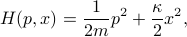
where $p = m frac {dx}{dt}$ is the momentum. If we were in a mechanics course, we'd solve Hamilton's equations and find the time-trajectory of how the particle moves around. But we're in a thermodynamics course, so instead, we want understand the thermal behavior of the system. Rather than seeing how the isolated system evolves, we're going to couple it to a big heat bath, wait for a long time, and ask the question ‘‘how often does it spend time in a particular configuration of and ?’’ (Physically, we can imagine the heat bath as bunch of molecules bumping into the particle, delivering little kicks that cause its energy to fluctuate around.)

If we wait for long enough, our poor bombarded particle will reach thermal equilibrium, where the probability it has some energy is proportional to $e^{-beta E} / Z$ (with beta the inverse temperature). The normalization constant is given by the summing up $e^{-beta E}$ over all possible configurations of the harmonic oscillator. Since we're considering a classical harmonic oscillator, we have to sum over all positions -infty < x < infty and all momenta -infty < p < infty . We can think of this as an integral over phase space (x,p) .

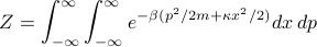
So we need to perform the following integral to find the partition function:

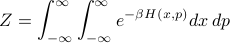
$Z = int_{-infty}^{infty}int_{-infty}^{infty} e^{-beta H(x,p)} dx , dp$

Plugging in the quadratic form of the Hamiltonian, we get

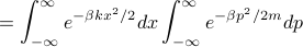
$Z = int_{-infty}^{infty}int_{-infty}^{infty} e^{-beta (p^2 / 2m + kappa x^2 /2)} dx , dp$

$quad = int_{-infty}^{infty} e^{-beta kx^2 / 2} dxint_{-infty}^{infty} e^{-beta p^2 / 2m} dp$

Lo and behold, it's just the product of Gaussian integrals that look like 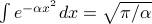$int e^{-alpha x^2} dx = sqrt{pi / alpha}$ , so the partition function is straightforward to find:

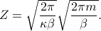
$Z = sqrt{frac{2pi}{kappabeta}}sqrt{frac{2pi m}{beta}}.$

Remark

We've performed a classical integral over phase space, rather than a quantum mechanical sum over energy eigenstates! In honesty, there's very few classical systems that we can treat in such a thermodynamic manner, because if the system is small enough that the thermal fluctuations actually affect its motion, then it's probably small enough that the quantized energy levels matter. (For instance, the vibrational energy levels of a simple diatomic molecule have an energy spacing comparable to room temperature.) And if the energy gaps are a comparable size to the thermal energy , then the classical phase-space integral is not appropriate, and we need to perform a quantum mechanical sum-over-states instead.

So what sorts of physical situations would this sort of treatment be appropriate for? An example I can think about is a bead held in an optical trap – the bead is massive enough that we won't have to care about its quantized energy levels, but the potential is shallow enough that we can see its Brownian motion as it's constantly bombarded by the molecules in its environment.

Finding the spread

In mechanical equilibrium, the particle settles down and stops moving at the minimum of the potential energy; but in thermal equilibrium, it still fluctuates about the minimum because it's constantly being bombarded by things in the heat bath. A natural question to ask is the mean squared size of these fluctuations – thermal fluctuations cause the particle to wander from the minimum, so how far does it tend to wander?

Well, we should first check that the particle is centered around the minimum; that is, we want to make sure that langle x rangle = 0 . In fact, we can argue that the average position is zero without performing the integral, by the following symmetry argument. Remember that the thermal average is given by integrating against the probability measure 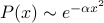$P(x) sim e^{-alpha x^2}$ , which is an even function. The expectation value of (an odd function!) looks like 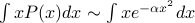$int x P(x) dx sim int x e^{-alpha x^2} dx$ . But since the integrand is odd, the half of the integral with x > 0 cancels out the part with x < 0 , and so the integral is zero. So indeed the probability distribution over is centered at 0.

However, the second moment langle x^2 rangle isn't going to vanish. In fact, we can find the spread in by staring closely at the Boltzmann factor $e^{-beta H(x,p)}$ . It tells you that the probability that the particle is at a position is given by

$P(x) sim e^{-beta kappa x^2 / 2},$

which has the form of a Gaussian (a.k.a. normal distribution). Remember that the standard form of a Gaussian with mean and variance sigma^2 is

$e^{-(x-mu)^2 / 2 sigma^2}.$

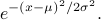
Comparing this standard form to our expression for P(x) tells us that the spread langle x^2 rangle is given by 1 / beta kappa = T / kappa . So we found the answer without doing any integrals (!).

Does this expression make sense?

As the temperature increases, the heat bath causes the oscillator to flail around more and more wildly, so it tends to wander further. Indeed .
As the stiffness increases, it takes more energy to climb further out the potential well, so the particle will tend to spend time closer to the center. Indeed .
The units are correct.

So great. The mean squared fluctuation in position is given by langle x^2 rangle = T / kappa . And thus we have solved the 1D harmonic oscillator.

Remark

Remember that the canonical ensemble is a probability distribution over points in phase space P(x,p) . However, here I've been talking about a probability distribution over position P(x) . Implicitly, what I've done is that I've integrated over the momentum to find the ‘‘marginal distrubtion’’ over position: P(x) = int P(x,p) dp . In fact, since there weren't any cross-terms between and in the Hamiltonian, the -distribution and the -distribution are actually independent of each other, so P(x,p) = P(x) P(y) . Yay, the joys of probability.

Generalizing to Higher Dimensions

Next up, we'll generalize a bit by considering particles that move in multiple directions. (If you don't mind, I'm also going to ignore the momentum part of the partition function as well, since it factors out. The distribution over is what we care about. See the remark box above.)

Let's go to three dimensions, and pretend that the particle's moving in a spherically symmetric harmonic well. Now it feels a potential of

$V(r) = frac kappa 2 r^2,$

where r^2 = x^2 + y^2 + z^2 represents your typical radial coordinate. If we squint at the expression for V(r) a little bit, we realize that each of the dimensions appears independently. That is, we can write it as

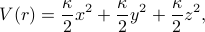
$V(r) = frac kappa 2 x^2 + frac kappa 2 y^2 + frac kappa 2 z^2,$

which we can recognize as the sum of independent harmonic oscillators in each spatial dimension. So each component of the particle behaves exactly like 1D harmonic oscillator! For instance, we can automatically deduce that 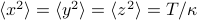langle x^2 rangle = langle y^2 rangle = langle z^2 rangle = T / kappa , and hence langle r^2 rangle = 3 T / kappa . We can also deduce that $Z_{3D} = z^3$ , where $Z_{3D}$ is the 3D partition function and is the 1D partition function. (If you don't believe me, you can try working out the calculations and convincing yourself.)

Remark

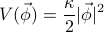
This is an example of the equipartition theorem of classical statistical mechanics: each quadratic degree of freedom contributes an amount $frac 1 2 kT$ to the thermal energy. In this case, each dimension of the harmonic oscillator counts as a separate degree of freedom, because it adds something like u^2 to the Hamiltonian.

Before going on, let's introduce some further notation to generalize to dimensions. Rather than calling the displacements in each of the directions as , , and , let's call them phi_1 , phi_2 , and phi_3 .In this language, the potential energy is given by

$V(r) = frac kappa 2 (phi_1^2 + phi_2^3 + phi_3^3) = frac kappa 2 sum_{a=1}^N phi_a^2.$

To be explicit about the notation: the symbol phi_a represents the displacement of the particle in the -dimension. The index labels each of the dimensions (for instance, in N=3 dimensions, we're summing over the , , and directions). And the quantity sum_a phi_a^2 represents the ‘‘radial’’ distance from the center of harmonic potential well, in analogy with the standard r^2 = x^2 + y^2 + z^2 .

To save a bit of space, we can also use vector notation vec phi where the length of the vector is given by vec phi cdot vec phi = |vec phi|^2 = sum_a phi_a . Then the harmonic potential is

$V(vec phi) = frac kappa 2 |vec phi|^2$

Keep this notation in mind, because it only gets more confusing.

Generalizing to multiple harmonic oscillators

Now let's pretend that rather than just having one single harmonic oscillator, we have multiple harmonic oscillators. Well, we can label each of our oscillators with an index , and write the displacement of the 'th oscillator as phi_i . If we have a total of oscillators, then the total potential energy is given by summing up the potential energy of each individual oscillator:

$V = frac kappa 2 |vec phi_1|^2 + frac kappa 2|vec phi_2|^2 + ldots + frac kappa 2|vec phi_L|^2 = frac kappa 2 sum_{i=1}^M |vec phi_i|^2$

Now we see why the notation gets kind of hairy. The index on the phi is labels which oscillator we're looking at, whereas the vector symbol on top of the phi refers to the directions of displacements of each of the oscillators. Hopefully it's not terribly confusing.

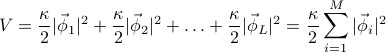
Thankfully, apart from the notional headaches, the thermodynamics of this problem very straightforward, since none of the oscillators are interacting with each other. Each of the oscillators lives in its own world, so its expectation values and partition functions are exactly the same as in the single-oscillator case. To be explicit, langle vec phi_i rangle = 0 for all the different sites , because each of the oscillators is centered around zero-mean-displacement. And 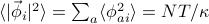$langle |vec phi_i|^2 rangle = sum_a langle phi_{ai}^2 rangle = N T / kappa$ , where is the number of dimensions. (Convince yourself why this is true!)

This is all quite straightforward so far. Let's make things a bit more exciting by allowing the oscillators to interact with each other.

Coupled Harmonic Oscillators

Now we're going to go through the classic derivation of finding the normal modes of a chain of balls and springs. We'll see that the energy separates nicely into a sum of Fourier modes. Once understand how this works, the Gaussian model that we did in class will follow pretty easily.

This derivation is typically done in a first course in thermodynamics, or in an advanced mechanics class…it's the problem of finding the vibrations of a periodic lattice, such as the atoms in a crystal.

Problem Statement

Here we'll consider a chain of coupled 1D harmonic oscillators in one dimension. You can imagine this as a long line of masses, with springs connecting the masses. If you pick up one of the masses and jiggle it around, the other masses nearby start moving around in a pretty complicated manner, and eventually, through all the couplings, the whole system of masses and springs will be vibrating in all sorts of complicated ways.

Our goal here is to simplify this complicated motion into a sum of simple ‘‘basis’’ motions.

1D chain

Consider a chain of masses, each spaced a distance apart. For simplicity, pretend that the masses live on a loop (i.e. periodic boundary conditions), so that mass #N is connected back to mass #1. Each mass is moving in its own harmonic potential with spring constant . In addition, each pair of neighboring masses is connected with a spring with spring contant .

The potential energy is given by

$V = frac mu 2 sum_j phi_j^2 + frac J 2sum_j (phi_j - phi_{j-1})^2,$

where phi_j is the displacement of the 'th mass from equilibrium. Here the first term represents each mass's own potential, and the second term represents the restoring force between two neighboring masses that are closer or further than the equilibrium separation.

Our goal is to find the thermodynamic quantities of this model. In particular, we want to find the two-point correlator langle phi_i phi_j rangle , which tells us how much the displacements at site and at site are correlated in equilibrium.

Let us write out the energy more explicitly so that we have a better idea what's going on. If we have L=4 masses, then it looks like

$V = frac mu 2 phi_1^2 + frac mu 2 phi_2^2 + frac mu 2 phi_3^2 +frac mu 2 phi_4^2 frac J 2 (phi_1 - phi_2)^2 + frac J 2 (phi_2 - phi_3)^2+ frac J 2 (phi_3 - phi_4)^2 + frac J 2 (phi_4 - phi_1)^2$

$V = left(frac mu 2 + J right) phi_1^2 + left(frac mu 2 + J right) phi_2^2 + left(frac mu 2 + Jright) phi_3^2 + left(frac mu 2 + Jright) phi_3^2 - J phi_1 phi_2 - J phi_2 phi_3 - J phi_3 phi_4 - J phi_4 phi_1.$

Notice that we have cross-terms between the phi's such as phi_1phi_2 . Because of these cross-terms, we won't be able to factorize the integrals int ldots dphi_1 , dphi_2 , dphi_3 , dphi_4 to find the partition function. So we'll need to find a way to rewrite the energy so that there's no more cross terms.

Here's the trick: we'll perform a Fourier Transform. If we write the energy in terms of the amplitudes of Fourier modes, rather than the displacements of particular sites, then there's no more cross terms. In the language of quantum mechanics, the Hamiltonian is diagonal in the momentum basis rather than the position basis.

Since we're going to perform a change of basis, let us use the language of linear algebra.

Thinking in terms of linear algebra

The configuration of our system – the state of all the springs and masses – lives in an -dimensional space (because you need different numbers to fully specify its state). And just like any vector space, you can represent your state in any basis you'd like. Currently we're using the position basis [phi_1, phi_2 ,phi_3 ,phi_4] to specify state of the system.

When we write our configuration using the position basis, it's easy to interpret the state vector, because each of the components are just the displacements of individual oscillators – the first component phi_1 is the displacement of the first oscillator, etc. However, the position basis has the downside that the Hamiltonian is not diagonal in this basis. That is, there are cross-terms between the different positions such as phi_1 phi_2 . This non-diagonal-ness is more clear when we write out the energy in matrix notation as

$V = left[ begin{array}{c} phi_1 phi_2 phi_3 phi_4 end{array} right]^T left[ begin{array}{cccc} frac mu 2 + J & -frac J 2 & & -frac J 2 -frac J 2 & frac mu 2 + J & -frac J 2 & & -frac J 2 & frac mu 2 + J & -frac J 2 -frac J 2 & & -frac J 2 & frac mu 2 + J end{array} right] left[ begin{array}{c} phi_1 phi_2 phi_3 phi_4 end{array} right].$

In this expression we explicitly see that the quadratic form has non-diagonal elements, which causes terms such as phi_1 phi_2 to appear in the energy.

If we instead chose a different basis to represent the energy, where the coupling matrix was diagonal, then we'd get rid of all the cross-terms, so we could easily calculate the partition function. That is, if we switched into a new basis [Phi_0, Phi_1, Phi_2, Phi_3] where the energy looks like

$V = left[ begin{array}{c} Phi_0 Phi_1 Phi_2 Phi_3 end{array} right]^T left[ begin{array}{cccc} # & & & & # & & & & # & & & & # end{array} right] left[ begin{array}{c} Phi_0 Phi_1 Phi_2 Phi_3 end{array} right],$

then we'd be in business, because there would be no more cross terms like Phi_2 Phi_3 . (Take a moment to convince yourself why this is true…)

In principle, to find this nice new diagonal basis, we need to find the eigenvectors of the -by- coupling matrix. However, we don't actually have to do any hard work, because we know that the answer is the Fourier basis 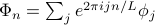$Phi_n = sum_j e^{2pi i j n / L} phi_j$ . Perhaps I can provide some justification for why this answer is physically reasonable.

Coming soon….

The Gaussian Model

Alas, I'm getting a bit lazy, and I'm not sure if I'll be able to muster the motivation to finish up the rest of this page. I'll summarize the main points behind this model and just wrap things up.

For simplicity I'm just working in one dimension….it's rather straightforward to tack on the indices to generalize to higher spatial dimensions (and phi dimensions). The only tricky part is recovering the real-space correlation function via inverse Fourier Transform, and thankfully, I think Jack our ever-helpful TA will be putting up a helpful worksheet on that later this week!

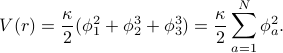
Written in terms of the Fourier modes , the total energy no longer has any cross-terms between modes of different wavenumber . We can write it as

$V = frac 1 2 sum_k (Jg(k) + mu) |Phi_k|^2,$

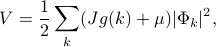
where the structure factor 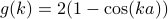g(k) = 2(1 - cos (ka)) is related to the local structure of the energetic couplings. Notice that g(k) approx k^2 for small , which means that g(k) to 0 as k to 0 .

Notice that the energy is a sum over the Fourier modes (labeled with ), and that the amplitude of each mode appears squared. The factor in front of of the tells you how ‘‘stiff’’ the 'th mode is. There are two contributions to stiffness: one is the intrinsic stiffness of individual oscillators , and another is a wavenumber-dependent term that goes to zero for long-wavelength excitations (small ).
Since the energy separates into a sum over modes, we know that the vibrations of different modes are uncorrelated to each other; that is, $langle Phi_k Phi_{k'} rangle = 0$ if . So once you look at the problem in the Fourier basis, the whole mess of coupled springs turns into a bunch of non-interacting harmonic oscillators.
For a particular normal mode of wavelength , the energy looks like 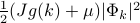$frac 1 2 (J g(k) + mu) |Phi_k|^2$ , which tells you it acts like a harmonic oscillator with spring constant 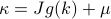. Since the modes don't interact with each other, we can quote our result from the earlier ‘‘simple harmonic oscillator’’ problem to say that

$langle |Phi_k|^2 rangle = frac T kappa = frac T {J g(k) + mu} , longrightarrow , frac T {J k^2 + mu} , textrm{when } k to 0.$

Look, ma, no integrals!

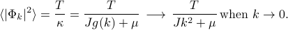
How excited are different modes?

The long-wavelength plane waves (small ) are the lowest energy excitations, so most of the thermal energy goes into these degrees of freedom. The shorter-wavelength, higher-frequency waves are much ‘‘stiffer’’ and tougher to excite, and thus they have a smaller mean squared amplitude at thermal equilibrium.
Notice that the mean squared excitation of the mode diverges when we set ! (Remember that .) Since fluctuations become more and more important near critical points, we are tempted to say that corresponds to a critical point. However, since the Gaussian model doesn't make any sense for , we can't actually learn about how the ordered phase behaves from this model. We can only learn about the behavior of the disorderd phase as it approaches the continuous transition.
- Later on we will use this model as a variational guess in order to derive some critical exponents that extend beyond mean-field theory.

The correlation length

Notice that there are two terms on the bottom of the fraction, the term and the term. If is big, then the first term's bigger; if is small, then the second term's bigger. The crossover point when the two terms are equal happens when or when .
Remember that the wavenumber has units of inverse length. (For instance, the wavelength is given by , so must have units of one over length for the wavelength to have units of length.) Taking the inverse of this ‘‘crossover ’’ gives us the characteristic lengthscale of the problem , known as the correlation length.
- Behold the power of dimensional analysis…
In fact, this is a rather powerful result! Since the correlation length is the only possible quantity that we can construct with units of length, we know that every spatially-dependent phenomenon in this problem occurs on a lengthscale of . For instance, the correlation between two points…

Finding the real-space correlation function

In real life, we don't just care about Fourier space, we also care about position space as well. It may be mathematically convenient to express energies in terms of sums over wavenumber rather than sums over position , but at the end of the day, if we wish to do any local experiments probing different parts of materials, we better express physical quantities in terms of .
One particularly interesting quantity is , which tells you how much the fluctuations at site are correlated with the fluctuations at some other site .
- Because of translational and rotational invariance, we expect taht this correlation function only depends on the distance between the sites .
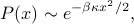
- Furthermore, from our result with the 1D Ising model, we expect that at long enough distances, the correlation should decay exponentially with a characteristic lengthscale of (because it's the only lengthscale in the problem)!
- Again, as we approach a critical point, we expect that sites which are further and further away become more and more correlated, because once we're in the ordered phase, faraway sites point in the same direction and thus are correlated. This means that the correlation length probably diverges at the critical point.
To calculate the real-space correlation function, we can express the displacements as a sum over Fourier modes 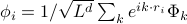$phi_i = 1/sqrt{L^d} sum_k e^{i k cdot r_i} Phi_k$ , and then use our knowledge about to simplify the result.
- The result looks like the Fourier Transform of a Lorentzian, which is indeed a decaying exponential at large distances…

Gaussian Model

Why study the Gaussian Model?

Why is the Gaussian Model solvable?

Game Plan

Outline

The Harmonic Oscillator

Finding the spread

Generalizing to Higher Dimensions

Generalizing to multiple harmonic oscillators

Coupled Harmonic Oscillators

Problem Statement

Thinking in terms of linear algebra

The Gaussian Model

How excited are different modes?

The correlation length

Finding the real-space correlation function

Leave a Comment Below!