Mean Field Solution of Ising Model
Now that we understand the variational principle and the non-interacting Ising Model, we're ready to accomplish our next task. We want to understand the general d-dimensional Ising Model with spin-spin interactions by applying the non-interacting Ising Model as a variational ansatz. In other words, we want to use what we just derived for independent, uncorrelated spins as a trial Hamiltonian in a variational treatment of the full Ising model.
As we'll see, we'll be able to interpret our results as a mean-field model, where each of the spins on the Ising lattice experiences the ‘‘average’’ field produced by all its neighbors. We'll discuss whether or not this brutal averaging is justified, and talk about under what circumstances it's more or less reasonable.
As an added bonus, we'll also encounter our first example of a continuous phase transition. In this dramatic process, the spins go from a disordered random phase with no overall magnetization to an distinct low-temperature ordered ferromagnetic phase where a macroscopic fraction of the spins are all aligned in the same direction. It's really quite surprising that Nature exhibits these sorts of marvelous ‘‘collective conspiracies’’, and it's even more surprising that they occur at a single well-defined temperature called the critical temperature  .
.
Finally, we'll talk about how to figure out the value of the critical temperature by drawing a picture and seeing where two graphs intersect.
Okay let's get started.
We solved the 1D Ising model by using transfer matrices…but why can't you solve the general n-dimensional Ising model with transfer matrices?
Variational Solution to Ising Model
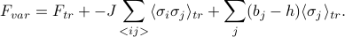
The game plan for today is to solve the general Ising model
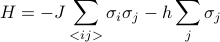
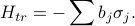
by using a trial Hamiltonian of the form
Here our full Ising model has an energetic coupling between neighboring spins  and
and  and the external field
  acting on all the spins. In our variational ansatz
  , we pretend that the spins are actually decoupled from each other (that is, there's no
  terms), and that each of the spins instead experiences an ‘‘effective external field’’
  . (We'll discuss how to interpret later on.)
Our objective here is to find the values of that make our trial Hamiltonian the ‘‘best’’ possible approximation to the actual Hamiltonian. As we learned, the variational principle says us that the ‘‘best’’ value of is the one that minimizes the variational free energy

(Remember that the subscript  means that we're finding thermal averages using the weights from the trial ensemble. This statement is much fancier than it sounds; it just means that whenever we see something such as
  , we just replace it whatever the solution to the trial Hamiltonian was. For instance, in this example, we're using the non-interacting Ising model as a trial Hamiltonian, so we plug in the formulas at the bottom of the last page.)
Let's begin.
Finding the variational free energy
We have no recourse but to plug everything into the formula for  . We find that
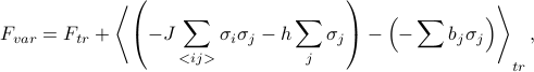
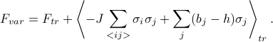
or combining terms,
And since expectations values are linear, we can pull the expectation values inside to go around the sigmas. (If you want to convince yourself of this, you can try writing out the difinition of  .)
.)
Before moving on, we can make one more simplification: since we picked a non-interacting trial Hamiltonian, the spins are uncorrelated, so  just factors into
  . (We can't always do this; we just happened to pick a non-interacting trial Hamiltonian today.)

(I changed the labels of the indices in preparation for the next step where we differentiate w.r.t. .) At this point, we can expand out our expressions for  and
and  , but a lot of the terms will cancel out later on, so for now, we'll just leave this expression as it is. (Prof. Kivelson calls this ‘‘being clever,’’ but I call it ‘‘hindsight is 20-20.’’)
Finding the derivative
Since we want to minimize with respect to the variational parameters , we just take the derivative and set it equal to zero. Nothing particularly fancy here yet. For now, we'll leave everything in terms of 's because we're ‘‘clever.’’
When we hit with a  :
:
The first term gives us a
 . You can see this is true by plugging in
  and then expanding out the partition function…or if you want some thermodynamic justification, read the Remark at the bottom of this page.
For the second term, the derivative only hits the terms involving spin
 , because the trial Hamiltonian only had terms which looked like
  . In the nearest-neighbor-sum, there is one term for each nearest neighbor of site , so we end up with a sum over nearest neighbors
  of
of 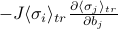
In the last term, we use the product rule. When we hit the coefficient, we get
, and when we hit the sigma we get 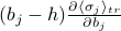 .
.
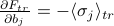
So the derivative of the variational free energy ends up being
where in the second sum, I'm summing over sites that are nearest neighbors (n.n.) of site .
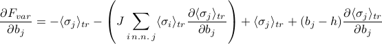
Now time for some magic: the first and the third term cancel out, and then we can factor out a  from what's left! And then when we set the derivative equal to zero, we're left with
![0 = frac {partial F_{var}} {partial b_j} = left[-J sum_{i , n.n.,j} langlesigma_irangle_{tr} + b_j - hright] {partial langlesigma_jrangle_{tr} over partial b_j}](eqs/4342851219466996748-130.png)
or
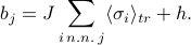
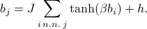
Finally, at this point we finally need to plug in our expression for  from the previous page; we end up with a relation between the external field of a spin and the external field of its neighboring spins
  .
.
Translational invariance
Hooray, we finally have an expression for the 's that satisfy our variational condition  . Unfortunately, all the 's are related to each other in a nasty sort of way involving hyperbolic tanhs, so it all looks kind of messy.
So to proceed further, we make the assumption of translational invariance that all spins really experience the same ‘‘external’’ field; i.e., that equals the same  for all the sites .
What's the motivation exactly for assuming  ? We tried to justify it in section by some argument about the zero-temperature limit, but I wasn't fully convinced, because the variational parameters depend on temperatures anyways.
A few weeks later in class, when we learned about Landau-Ginzburg theory, we were able to give a more convincing argument for why a spatially uniform solution for is indeed the ‘‘best’’ solution.
Once we assume that is the same for all sites, we can simplify our result quite a bit, because we only need to find one unknown now. The on the LHS is the same as on the RHS. Our sum over the nearest neighbors of site ends up being the same for each of its neighbors, so rather than summing, we just need to multiply by the number of nearest neighbors  .
.
These simplifications give as an equation for in terms of itself as
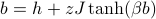
where is the number of nearest neighbors in the Ising model.
The number of nearest neighbors in an Ising model on a  -dimensional hypercube lattice is
  . For instance, on a chain (
 ), you have 2 neighbors to your left and right; on a square grid (
 ), you have 4 neighbors (left, right, up, down); on a cubic lattice (
 ), you have 6 neighbors (
 ), and so on and so forth.
It's confusing to write  because the little looks like a subscript on
  , which is reminiscent of the
  spin operator in quantum mechanics (and also reminiscent of a certain rapper…)
On the other hand,  means a zeptojoule or
  Joules! And wouldn't you know, the thermal energy
  is typically on the order of zeptojoules; at room temperature
  , it's roughly 4 zJ….I swear there's a conspiracy going on here.
Solving for b
At this point, we have an expression involving on the LHS and the RHS. If we think back to the bigger picture, we have just learned that the value of which satisfies this equation is the ‘‘best’’ possible value of in our trial Hamiltonian. Unfortunately, we can't explicitly solve for in a closed-form way…so how do we proceed further?
We'll appeal to the maxim: when in doubt, simplify things and draw a picture. So let's set  for now, and draw a picture, and see if we can gain any qualitative insight.
Our strategy here is to plot both sides of the equation and see where the graphs intersect. The intersection points will tell us the solutions for . In this case, we want to where the graphs of  and
and 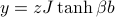 intersect:
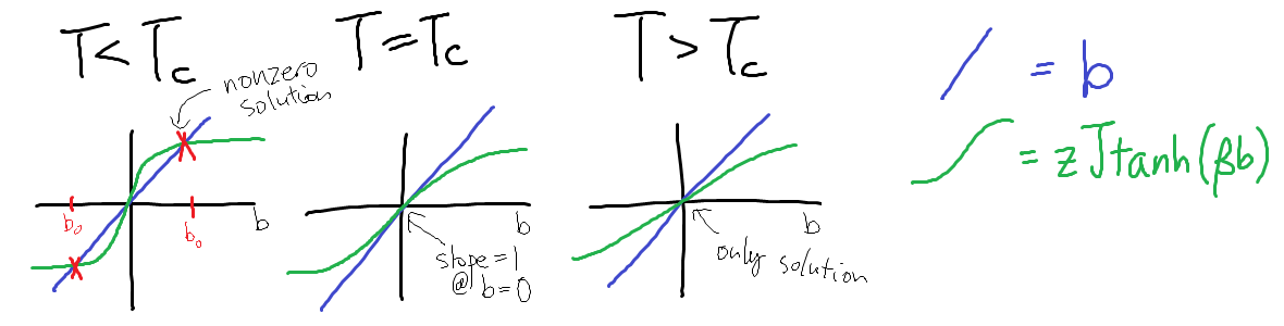
Surprisingly, the number of graph crossings depends on the temperature! This is by far the most interesting thing we've discovered in class so far: the behavior of the mean-field Ising model is completely different at low temperatures than at high temperatures. We've discovered a phase transition.
If you start out at high temperature, you'll only find a trivial solution at  , but when you lower the temperature past a special critical temperature , all of a sudden, there will be nonzero solutions
  as well. This is rather remarkable; it tells us the system behaves dramatically differently depending on whether
  or
or  . The high-temperature regime is called the paramagnetic phase and the low-temperature regime is called the (anti)ferromagnetic phase.
Physical interpreation
Let's think back to our main physical observable, the magnetization density  which tells us whether the spins tend to align up or down in thermal equilibrium. (To calibrate our intuition, it's helpftul to review how non-interacting spins behave at different temperatures.)
In our mean-field model, the magnetization density is given by  , which means at low temperatures when is nonzero, there is a net nonzero magnetic moment in the system.
Wait a second. Let's think about how unusual this is. Since we dialed down the external field to zero, there is no energetic incentive whatsoever for the spins to want to align one way versus another. There's nothing pulling on the spins to make them want to point in a particular. Yet we've just discovered that there's a nonzero net magnetic moment at low temperatures; in other words, that all the spins are preferring to point in some direction over the other! How is this possible?
Well, believe it or not, this is how nature behaves. It's what you might call a collective conspiracy – none of the individual spins feel an external field, but if enough of them happen to fluctuate and point in a particular way, they'll set up a strong enough ‘‘local field’’ to convince their neighbors to the same way – so strong, in fact, that a nontrivial fraction of the  spins also ‘‘get in on the conspiracy’’, and the material develops long-range order and gains a macroscopic magnetic moment. Truly remarkable, especially if you consider just how many spins there are (
 ), and just how weak each individual magnetic moment is. Magical.
So to summarize, we've just discovered a conspiracy:
At high temperatures
, the spins exhibit a disordered paramagnetic phase, pointing in every which way. The average magnetization of the system is zero.At low temperatures
, the spins exibit an ordered ferromagnetic phase, where they all conspired to point in one direction (even when there's no external field telling them which way to point!) The average magnetization of the system is (shockingly) nonzero.
How come long-range order only develops at low T?
Here is a qualitative picture for why high temperature favors disorded phases. At sufficiently high temperatures, all the spins are jiggling around with so much thermal energy that any local conspiracies of all-up-zones or all-down-zones are quickly jiggled away out of existence before they have time to spread into a macroscopic fraction of the material.
There's also a nice argument that comes from the interplay between the two terms of the free energy  . Each phase has its own energy
  and entropy
  , and depending on the value of the temperature
  , the free energy
  of one phase might be higher than the other.
In the disordered paramagnetic phase, the spins can point in any which way, so there's lots of possible configurations (high entropy, favorable), but there's very little energetic reward because the spins haven't chosen to align (high energy, unfavorable).
In the ordered ferromagnetic phase, the spins have all conspired to point (mostly) in one direction, so there are less possible configurations for them (low entropy, unfavorable) but since they're neatly lined up in an energy-minimizing manner, there's a glorious energetic reward (low energy, favorable)
Which phase has the lower free energy? At high temperatures, when the entropic contribution is more heavily weighted, the paramagnetic phase flies off to an entropic heaven of possibilities, whereas at low temperatures, when all the system wants to do is to minimize energy, the orderly ferromagnetic phase wins out.
Solving for the critical temperature
Alright, enough qualitative remarks, I'm starting to sound like a chemist. Let's move on to solve for the critical temperature  .
.
Let's look at our pictures again:
Our goal here is to find the special temperature that separates the nonzero-solution-regime from the no-nonzero-solution-regime (sorry, these words are confusing). There's a simple condition that tells you whether or not the green curve will hit the blue curve again after . Can you figure it out by staring at the picture?
Here's the secret: The green curve has to be steep enough at for the blue curve to ‘‘catch up to it’’ later on and intersect the green line again. If the green line's steeper than the blue line at , then there'll be a nonzero solution for , and if it's shallower, there won't be. And if the green line is exactly as steep as the blue line at , then we're at the critical temperature that separates the two possibilities. Clever, eh?
This little observation gives us a mathematical procedure to find the critical temperature: we take the derivative of the LHS and RHS, set them equal to each other at , and solve for  . The slope of the blue curve
  is 1, and the slope of the green curve at is
![left[{partial over partial b} zJ tanh(beta b)right]_{b=0} = left[frac {zJbeta} {cosh^2 (beta b)}right]_{b=0} = z J beta.](eqs/5126426440385481560-130.png)
When we set the two slopes equal to each other, we find that  or
or  .
.
Continue to interpreting the mean-field solution.
Why does taking a derivative of the free energy w.r.t. the external field give you the magnetization ?
Well, you can see this directly by plugging in  and then expanding out the partition function. It's a pretty fun exercise to work this out yourself…remember that
  …
…
If you're feeling more thermodyanmically inclined, you can also convince yourself that  via the following thermodynamic argument. (Now I'm calling the external field
  and the magnetization
  in the true thermodynamic spirit.)
When we include the external magnetic field into a thermodynamic treatment, our internal energy function  gains an extra parameter . The external field gives us another handle to perform work on the system; when we twiddle it by an amount
  , the energy of the system changes by an amount
  , where we recognize the magnetization
  as the conjugate variable to the external field . (Think back to E'n'M why magnetic dipole times magnetic field gives you an energy…)
Once we include a magnetic field, we can either change the internal energy by adding some heat  or by performing some magnetic work
  , which means that the total differential of the internal energy is

However, since we're considering the Ising model in a canonical ensemble at a fixed temperature , it doesn't make much sense to talk about derivatives of the (internal) energy , because is a natural function of the entropy rather than the temperature . So even though we can find the magnetization in principle as a derivative of the internal energy as  , it's pretty physically useless to do so, because that derivative holds entropy constant rather than the temperature.
To account for this issue, we perform a Legendre transformation to the free energy

which then becomes a natural function of the temperature as  . The differential of free energy can then be expressed as

from which we can read off the magnetization
where the derivative is now taken at a fixed temperature rather than at fixed entropy, meaning that it aligns with our treatment of the Ising Model in the constant-temperature canonical ensemble of statistical mechanics.
Okay, to be fair, I didn't really prove anything in the above, I just kind of pulled the  term out of thin air and then waved my hands around for a sort of ‘‘plausibility’’ argument. But I do think it's a reasonable sort of thing to say. Hooray, thermodynamics.