Non linear techniques (continued)

The hybrid method
It resulted from our analysis of the methods we implemented that some of
them were doing better on specific kind of neighborhoods, like smooth
areas,
high contrast areas, textured areas or edge areas. For example, the following image shows the points where the
Cubic Spline method is doing best than the other methods. Although pretty
noisy, it shows that black dots are statistically more concentrated around
edges.
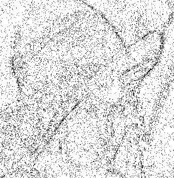
figure:pixels where the Cubic Spline method is optimal
It seems that we could take advantage of this statistical non-uniformity
by switching the method from one part of an image to the other,
depending on which one is expected to do the best job for each part
of the image. Then, we would be able to gain some prediction accuracy over the previously best method provided that this latter one is not optimal everywhere.
Image partitioning
This method requires to be able to classify the pixels of the
image into a set of neighborhood types. This partition of the image is
not necessarily related to the way we divided it into cells for the Approximated Optimal
NL method described before. However, using the exact same partition makes
it possible to keep together the pixels of the cells where the latter prediction does a very bad job
(due to the lack of training samples for that cell). For that reason, we
chose to use the same features and quantization as for the
Optimal NL interpolation.
The training scheme is described on the following diagram: for each
cell, we compute the average MSE of each method on the training image
set, and build a table to store the index of the method minimizing the
MSE.
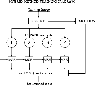
figure: Hybrid interpolator training scheme
Expected improvements
It seems clear that if the training is done using the image we intend
to use as a test, the hybrid method will systematically do better than
the best of the methods involved, because we reach the minimum MSE for
each of the cells. Nevertheless, in the general case (an image not included
in the training set), there is no guaranty that we will choose the optimal
method for each cell. The expected improvement rely on the fact that if
the cells' partition is sound, the methods' MSE ordering on each cell will
be almost unchanged from one image to the other. That is, the best method
table will generalize well to new images.
Choice of a common Reduce function
We once again have to choose one Reduce function as a common basis
for all the methods. Indeed, we can not change the
Reduce function from one cell to another because this would result in cross-cell
interactions in the Expand phase. Consequently we will not be able
to get the best from each method since most will not be used with their matching Reduce
function.
Implementation
We used the same parameters as for the Approximately Optimal NL method
described above, that is
-
Optimal Cubic decimation
-
Average intensity and gradient features
-
Non-uniform 8 level quantization for each of the features
The Expand methods we compared are :
-
Haar
-
Burt and Adelson with a=0.4 and 0.6
-
Ideal
-
Optimal Linear and Cubic
-
Linear and Cubic Spline
-
MMF
-
Approximated Optimal NL (as described in the last part of the previous page).
We got the following method map for the Lena image. It appears that Optimal
NL method is used for the major part of the image. Cubic Spline seems
to do a good job on edges,
while Optimal Cubic is best for textured areas. The hybrid method yielded
a 17.67 MSE, which is not a great improvement compared the Optimal NL
method.
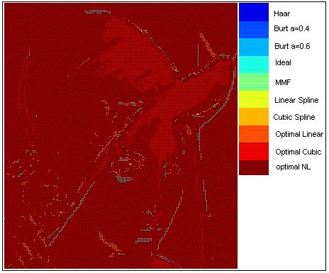
figure: method mapping on the Lena test image
Previous (Non Linear techniques)
Next (Visual Results)
