Linear techniques

We first considered a set of linear techniques for the main reason that they allow a systematic analytical approach.

We considered only 2-D separable filters, i.e. that can be expressed as the product of two 1-D kernels of width k.

It allows a stronger analysis because we have powerful tools to construct 1-D filters. As long as we are not interested in any kind of orientation analysis, this approach is perfectly sound although sub-optimal (otherwise circularly symmetric kernels would be necessary).

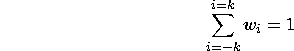
We concentrated on a subset of the 2-D separable filters verifying the following properties :

symmetry : both halves of the neighborhood affect the pixel symmetrically

normalization : the reduced image maintains the average intensity of the original image

unimodality : the closer a value is to the pixel, the stronger it affects that pixel's value

"Haar" approach

REDUCE = EXPAND = top-hat function

Before the decimation, we simply take the average value of a square of four pixels. In the interpolation step, the neighboring pixels get replicated with no additional interpolation filtering.

Burt & Adelson approach [1]

REDUCE = EXPAND = Gaussian-like filter

The same weighting function is used for the REDUCE and the EXPAND operations. It is a 5-by-5 filter which depends on only one parameter : this class of filter is the only class of 5-by-5 separable filter verifying the three properties mentioned above.

Ideal filter

REDUCE = EXPAND perfect low pass filter with cut off frequency at pi/2

This method is ideal in the sense of the reconstruction of the frequencies comprised between 0 and pi/2. The image is first convolved by a sinc to prevent any aliasing ; the lower resolution image is then interpolated using the same filter to remove all the replications of the spectrum after up sampling.

Optimal polynomial filters [2]

REDUCE = pre sampling filter optimized to minimize the MSE considering the given REDUCE operator
EXPAND = piecewise polynomial interpolation

This approach fits a piecewise polynomial surface to the 2-D intensity function. The criterion for optimality is the minimization of the MSE between the fitted surface and the original image at the pixel points.
This approach is probably not optimal because minimizing the MSE does not necessarily result in the best subjective image quality. However it allows a systematic analysis.
The 2-D kernel is generated from the 1-D kernel. The REDUCE function generates a chain of piecewise polynomial segments with fewer points (due to the decimation) from the original one. The EXPAND function makes a polynomial interpolation to assign values to the missing points.

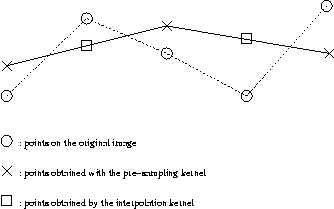
figure : 1-Dimensional linear piecewise fitting

This optimization involved in the decimation happens to have a solution that can be approximated by a trucated kernel convolution. We only considered two kernels : the linear and the cubic fitting kernels. The width can be specified : we chose filters with large width (15) to get better results. This is not damageable in terms of complexity since the EXPAND function is not affected by that choice.

Splines [3]

In [3], a scheme that generates a L2 polynomial spline pyramid is proposed. Polynomial splines of order n are piecewise polynomials that are connected to guarantee the continuity of the function and its derivatives up to order n-1. Splines are interesting for pyramidal coding for two reasons : first because it is possible to adjust the coarseness of the representation by varying the number of coefficients, thus enabling progressive data reduction. Secondly because discrete spline operations can be formulated in terms of separable convolutions (making by the way this scheme linear).

After a initial change of coordinates from image space to B-spline space (or dual space), the EXPAND and REDUCE functions can be expressed as simple FIR binomial filters. The changes in coordinates involve convolutions and inverse convolutions with the B-spline kernels of order n and 2n+1 : b(n) and b(2n+1). We approximated the inverse convolution by using a truncated FIR filter obtained by inverting the frequency response of b(n). The decimation and interpolation functions in 1-D are described below. The generalization to 2-D can done by successive 1-D processings along the coordinates.

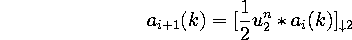
REDUCE:

EXPAND:

Comparison of the kernels used in REDUCE

The following figure summarize the properties of the different kernels we used for the REDUCE operator.

The plots of the frequency response is of particular interest. If we want to avoid aliasing in the decimation process, the filter has to be an ideal low-pass filter. All methods (except the ideal method) will experience some folding of the frequencies over pi/2.

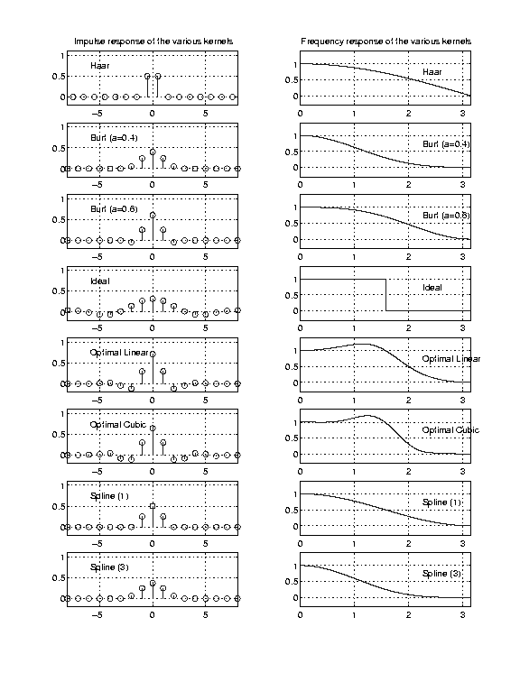
figure : comparison of the impulse and frequency response of the different filter kernels

The method of polynomials filter gives better results in terms of frequency response. The filter for the B-Spline should not be compared with the other since the filtering is done in the B_Spline space and not in the image space.

Previous (Introduction)-Next (Non-Linear techniques(1))