Due July 22nd, 11:59pm.
Written by Chris Piech.
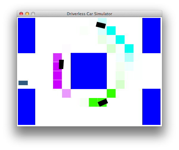
Figure 1: The Driverless Car project uses Hidden Markov Models, Exact Inference and Particle Filters.
Introduction
The development of a driverless car has many motivations -- perhaps the most important is to reduce the amount of road carnage. A new study by the World Health Organisation shows that such accidents kill a shocking 1.24m people a year worldwide. The hope is that by creating an AI agent that can drive, constantly aware and cautious, we could reduce the death toll.
In this project, you will design car agents that use a simple sensor to locate other cars and drive safely. You'll advance from driving blindly to tracking multiple other cars so that your car can make its way from start to finish accident free. In order to minimize financial costs, we are going to develop an autonomous car that uses only a microphone to sense other cars.
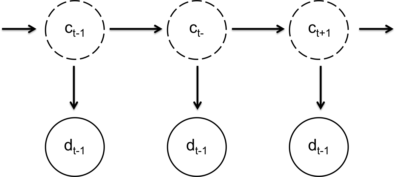
Figure 2: The hidden markov model that we are going to use to track cars. At each time point there is a hidden variable $c$ which is the actual location of the car and an observed variable $d$ which is a noisy sensor of the distance to the car (relative to your car).
The code for this project contains the following files, available as a zip archive.
Key files to read:
exactInference.py |
This is the file where you will program your exact inference algorithm. |
learner.py
| This is the file where you will program your learner, that observes cars and learns transition probabilities. |
particleFilter.py |
This is the file where you will program your particle filter. |
util.py |
Useful data structures for implementing search algorithms. |
Submission: Submission is the same as with the Pacman assignment. You will submit the files
exactInference.py,
learner.py and
particleFilter.py. See submitting for more details.
Evaluation: Your code will be autograded for technical correctness. Please do not change the names of any provided functions or classes within the code, or you will wreak havoc on the autograder. However, the correctness of your implementation -- not the autograder's judgements -- will be the final judge of your score. If necessary, we will review and grade assignments individually to ensure that you receive due credit for your work.
Academic Dishonesty: We will be checking your code against other submissions in the class for logical redundancy (as usual). If you copy someone else's code and submit it with minor changes, we will know. These cheat detectors are quite hard to fool, so please don't try. We trust you all to submit your own work only; please don't let us down. If you do, we will pursue the strongest consequences available to us, as outlined by the honor code.
Getting Help: You are not alone! If you find yourself stuck on something, contact the course staff for help. Office hours and piazza are there for your support; please use them. We want these projects to be rewarding and instructional, not frustrating and demoralizing. But, we don't know when or how to help unless you ask.
Tasks:
| Emission |
| Transition |
| Particle Filter |
| Driver |
Tasks
First, run a driverless car simulation with you behind the wheel. In general, your goal is to drive from the start to finish (the green box) without getting in an accident. How well can you do on crooked Lombard St without knowing the location of other cars?
python drive.py -l lombard
You can steer by either using the arrow keys or w, a, s, d.
Quit by pressing q
Without modeling where the other cars were, the staff was only able to get to the finish line 4/10 times. This 60% accident rate is substantially higher than the 300,000 miles the Google car is reported to have driven accident free.
1. Emission Probability
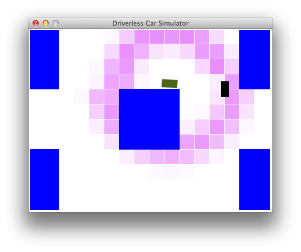
Figure 3: The probability of a cars location given an observation. When you finish this milestone you should be able to find a car by circling it.
Once a heartbeat (one update of our simulation) our microphone records how loud each car is, which we are then able to turn into a noisy measure of distance. According to the specifications, the microphone generates a distance observation (one for each car) $d$ that is distributed normally about the true distance $t$, with a standard deviation of Const.SONAR_STD (which if you are curious is about two thirds of a car length).
In the context of a hidden markov model, the probability of an observation given a current state is called the emission probability. Since our observation is generated using a normal, the emission probability is a normal probability density funciton (pdf). To get the probability of a normal distribution producing a value you can use the utility function util.pdf(mean, std, value).
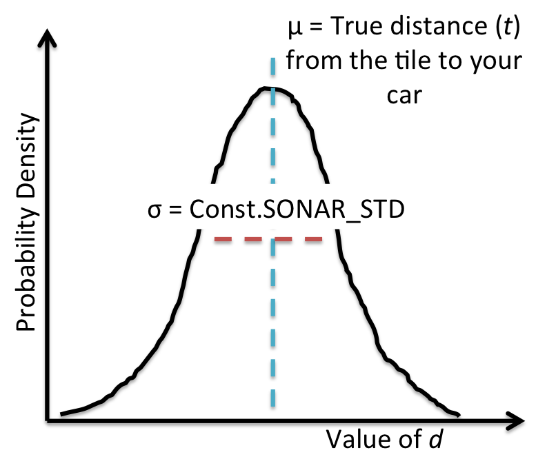
Figure 4: The probability density function for the sonar distance $d$.
Fill in the observe method in the ExactInference class of exactInference.py to update the probability of each tile given the observed noisy measurement. When complete, you should be able to find the location of a stationary car by circling it:
python drive.py -p -d -k 1 -i exactInference
util (similarly, given x and y you can calculate col and row). The observed distance from our microphone, and the location of your agent are reported in pixel units (x, y).
Update Equation: Before typing any code, write down the equation of the inference problem you are trying to solve.
Initial Belief: You are implementing the online belief update for observing new evidence. Before any readings, you believe the cars could be anywhere: a uniform prior.
For the People: A microphone only costs a few dollars.
2. Transition Probability
Fill in the carMove and the saveTransitionProb method in the Learner class of learner.py. Running the learner to completion took us 2 mins (it's important to see lots of different scenarios). If you want to test your code using fewer observations, you can change the learn settings in Const. Note that the structure of the dictionary you save is of your chosing!
python learn.py -l small
python learn.py -l lombard
Once you have learned the transition probabilities, finish ExactInference by writing the elapseTime method using your precomputed transition probabilities. You can load your saved transition probabilities (assuming that you created them) using util.loadTransProb(). If in your elapseTime method you come accross a tile that was never observed in training, you can assume that a car in this tile will not move. When you are all done, you should be able to track a moving car!
python drive.py -d -k 1 -i exactInference
-f turned on) and the car drives along the outer ring we get an error of 95.4 after 100 iterations and 72.5 after 200 iterations. When we grade your assignment we will run it multiple times with multiple different start conditions.
You have hit a major milestone. But what happens if you change the number of cars that you are tracking from 1 to 3? When you run exact inference on Lombard St
python drive.py -l lombard -i exactInferenceyour program may start to lag.
3. Particle Filter
ParticleFilter class in particleFilter.py. When complete, you should be able to track cars nearly as effectively as with exact inference.
getBelief, you must return a Belief instance (see util.py).
-p) and the display car flag (-d).
python drive.py -i particleFilter -l lombard
-d flag turned off.
4. Autonomous Driver (Optional)
getAutonomousActions method in AutoDriver has your car drive around haphazardly. The basic algorithm in the starter code AutoDriver is: Drive towards a goal node (in the underlying AgentGraph). Do not drive into any tiles where you have a reasonable belief that there may be a car. Once you have reached your goal, randomly chose a next state in the AgentGraph to be your new goal.
python drive.py -a -d -i particleFilter -l lombard
- Have the agent follow the shortest path to the terminal node (possibly using the
AgentGraph). - Program your agent to be careful of left turns where it could get side swiped. It might be useful to use your transition probability from part 2.
- The probability of an agent being in a tile is really the probability of the center of the agent being in the tile. Your agent should take into account the car width
Const.CAR_WIDTHto be perfectly safe.
Project 2 is done. Go Driverless Car!