Binary Table/Contingency Table representation
Reading in and forming tables from discrete data
A warm up problem: Plato’s sentence endings
��������������������������������������������������������������������������������������������������������������������������������������������������������������
> load("/Users/susan/sphinx/data/platofreq.RData")
> dimnames(platofreq)[[1]]=c("UUUUU","-UUUU","U-UUUU","UU-UU","UUU-U","UUUU-
",
+ "--UUU","-U-UU","-UU-U","-UUU-",
+ "U--UU","U-U-U","U-UUU-","UU--U","UU-U-","UUU--",
+ "---UU","--U-U","--UU-" ,"-U--U","-U-U-","-UU--",
+ "UU---","U-U--","U--U-","U---U","U----","-U---",
+ "--U--","---U-","----U","-----")
> apply(platofreq,2,sum)
Rep Laws Crit Phil Pol Soph Tim
3783 3788 150 957 772 919 765
> apply(platofreq,1,sum)
UUUUU -UUUU U-UUUU UU-UU UUU-U UUUU- --UUU -U-UU -UU-U -UUU- U--UU
219 316 260 255 313 344 308 249 173 655 419
U-U-U U-UUU- UU--U UU-U- UUU-- ---UU --U-U --UU- -U--U -U-U- -UU--
185 283 264 370 483 450 246 222 262 418 251
UU--- U-U-- U--U- U---U U---- -U--- --U-- ---U- ----U -----
332 265 650 259 396 423 368 701 285 510
> require(vcd)
Loading required package: vcd
Loading required package: MASS
Loading required package: grid
Loading required package: colorspace
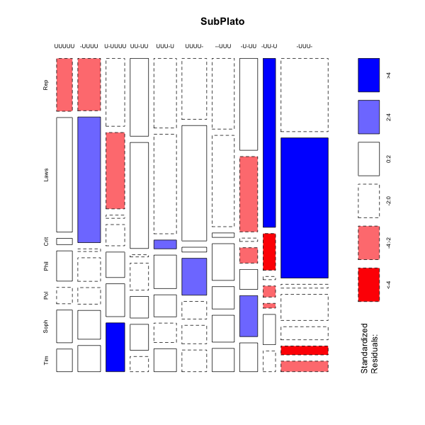
> mosaicplot(platofreq[1:10,],color=TRUE,shade=TRUE,main="SubPlato")
> require(ade4)
> res.plato=dudi.coa(platofreq,nf=2,scannf=F)
> res.plato
Duality diagramm
class: coa dudi
$call: dudi.coa(df = platofreq, scannf = F, nf = 2)
$nf: 2 axis-components saved
$rank: 6
eigen values: 0.09128 0.02121 0.009105 0.006023 0.002836 ...
vector length mode content
1 $cw 7 numeric column weights
2 $lw 32 numeric row weights
3 $eig 6 numeric eigen values
data.frame nrow ncol content
1 $tab 32 7 modified array
2 $li 32 2 row coordinates
3 $l1 32 2 row normed scores
4 $co 7 2 column coordinates
5 $c1 7 2 column normed scores
other elements: N
>
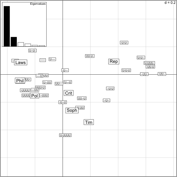
���������������������������������������������������������������������������������������������������������������������������������������������������������������������������������������������������������������������������������������������������������������������������������������������������������������������������������������������������������������������������������������������������������������������������������������������������������������������������������������������������������������������������������������������������������������������������������������������������������������������������������������������������������������������������������������������������������������������������������������������������������������������������������������������������������������������������������������������������������������������������������������������������������������������������������������������������������������������������������������������������������������������������������������������������������������������������������������������������������������������������������������������������������������������������������������������������������������������������������������������������������������������������������������������������������������������������������������������������������������������������������������������������������������������������������������������������������������������������������������������������������������������������������������������������������������������������������������������������������������������������������������������������������������������������������������������������������������������������������������������������������������������������������������������������������������������������������������������������������������������������������������������������������������������������������������������������������������������������������������������������������������������������������������������������������������������������������������������������������������������������������������������������������������������������������������������������������������������������������������������������������������������������������������������������������������������������������������������������������� > scatter(res.plato) >
The output of this correspondence analysis is the same as for a pca, the variance explained is replaced by the chisquare distance from independence explained.
What percentage of the total inertia is represented by this first plane?
> firstplane=round(sum(res.plato$eig[1:2])/sum(res.plato$eig),2)
> firstplane
[1] 0.85
>
We see that 85% of the total chisquare is explained by the first two axes. Beware if you use the function scatter on data tables with too many rows or too many columns the data become unreadable. We need a way of only projecting only columns or only rows.
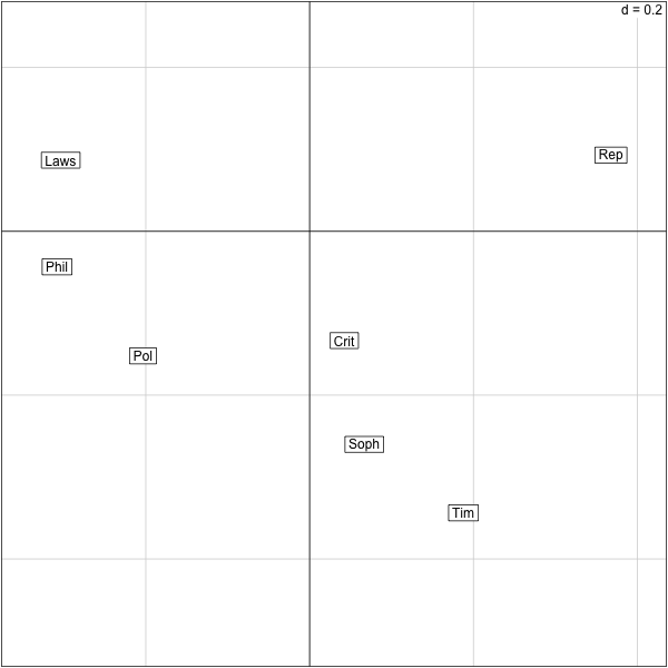
������������������������������������������������������������������������������������������������������������������������������������������������������������������������������� > s.label(res.plato$co) >
Some facts about tables and CA
- Often need to transform the original matrix of data to get the contingency table.
- Correspondence Analysis, homogeneity analysis is appropriate for binary or contingency tables.
- Gradients can be detected in the same way as in MDS (in fact CA is a type of MDS).
- The eigenvalues show how much of the Chisquare Inertia is explained by each successive eigenvector/axis.
- More Details in the Stats206 course notes.
Communities of species in Mice Gut Microbiome
With David Relman and Julie Theriot’s Labs we are studying the variability in mice gut ecological communities, we present here part of an analyses we did with Yana Hoy who kindly allowed us to share a subset of the data with you.
We are going to look at a set of mice at their resting states before intervention, however the mice are not homogeneous in many aspects. We want to study the baseline variability and the quality of the data before going further into the study.
The original data were passed through the usual qiime pipeline and the data were transformed into a read abundance table called py.nz.RData, contingent species (OTU) information is contained in the file otu.idy.RData. We load these files into the R workspace:
> load("/Users/susan/sphinx/data/py.nz.RData")
> summary(apply(py.nz,1,sum))
    Min.  1st Qu.   Median     Mean  3rd Qu.     Max.
     1.0      2.0     11.0    725.9    144.0 125200.0
>
We will do a correspondence analysis on the data using dudi.coa. We only plot the columns (mice), as there are too many taxa, what do we see?
������������������������������������������������������������������������������������������������������������������������������������������������������������������������������������������������������������������������������������������������������������������������������������
> res.py=dudi.coa(py.nz,nf=4,scannf=F)
> p1=round(100*sum(res.py$eig[1:2])/sum(res.py$eig))
> s.label(res.py$co,boxes=F,clabel=0.9)
> title(paste("Preinfected, axes 1:2",p1,"% inertia"))
>
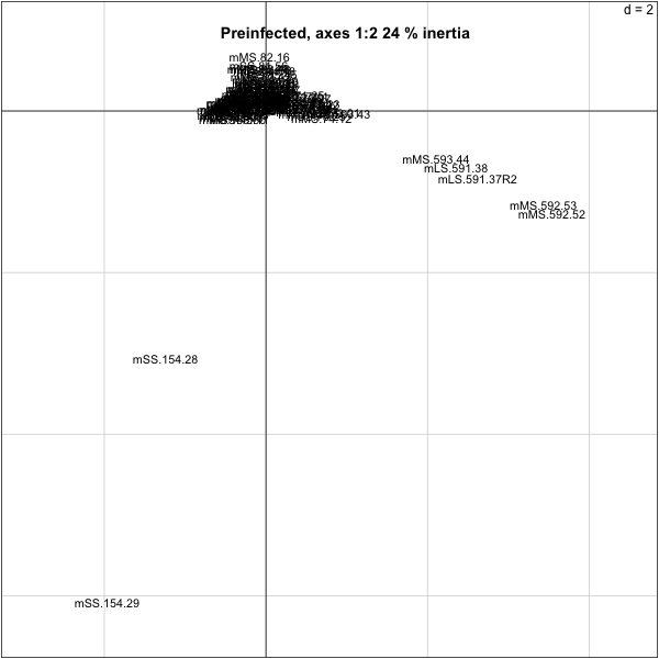
So we need to take out a few of the mice that are outliers:
���������������������������������������������������������������������������������������������������������������������������������������������������������������������������������������������������������������������������������������������������������������������������������������������������������������������������������������������������������������������������������������������������������������������������������������������������������������������������������������������������������������������������������������������������������������������������������������������������������������������������������
> py.nz.coa=dudi.coa(py.nz[,-(70:71)],scannf=F,nf=4)
> s.label(py.nz.coa$co,boxes=F,clabel=0.5)
> title("pre-inf. without 154.28 and 154.29,cols")
>
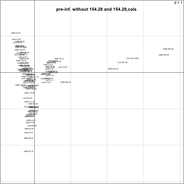
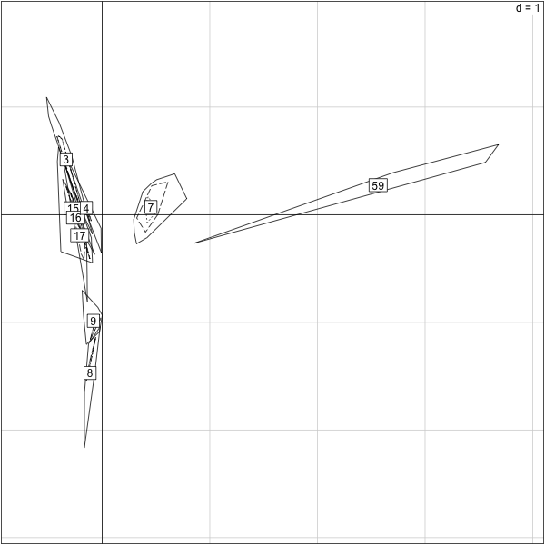
����������������������������������������������������������������������������������������������������������������������������������������������������������������������������������������������������������������������������������������������������������������������������������������������������������������������������������������������������������������������������������������������������������������������������������������������������������������������������������������������������������������������������������������������������������������������������������������������������������������������������������������������������������������������������������������������������������������������������������������������������������������������������������������������������������������������������������������������������������������������������������������������������������������������������������
> load("/Users/susan/sphinx/data/cage96.RData")
> cagelabel=factor(cage96[-(70:71)])
> s.chull(py.nz.coa$co,cagelabel)
>
R code for cut and paste
rm(X)
 load("/Users/susan/sphinx/data/platofreq.RData")
 dimnames(platofreq)[[1]]=c("UUUUU","-UUUU","U-UUUU","UU-UU","UUU-U","UUUU-",
 "--UUU","-U-UU","-UU-U","-UUU-",
 "U--UU","U-U-U","U-UUU-","UU--U","UU-U-","UUU--",
 "---UU","--U-U","--UU-" ,"-U--U","-U-U-","-UU--",
 "UU---","U-U--","U--U-","U---U","U----","-U---",
 "--U--","---U-","----U","-----")
 apply(platofreq,2,sum)
 apply(platofreq,1,sum)
 #Two dimensional summary
 require(vcd)
 mosaicplot(platofreq[1:10,],color=TRUE,shade=TRUE,main="SubPlato")
 require(ade4)
 res.plato=dudi.coa(platofreq,nf=2,scannf=F)
 res.plato
 scatter(res.plato)
firstplane=round(sum(res.plato$eig[1:2])/sum(res.plato$eig),2)
firstplane
 s.label(res.plato$co)
load("/Users/susan/sphinx/data/py.nz.RData")
summary(apply(py.nz,1,sum))
res.py=dudi.coa(py.nz,nf=4,scannf=F)
p1=round(100*sum(res.py$eig[1:2])/sum(res.py$eig))
s.label(res.py$co,boxes=F,clabel=0.9)
title(paste("Preinfected, axes 1:2",p1,"% inertia"))
py.nz.coa=dudi.coa(py.nz[,-(70:71)],scannf=F,nf=4)
s.label(py.nz.coa$co,boxes=F,clabel=0.5)
title("pre-inf. without 154.28 and 154.29,cols")
######First numbers in the label seem to group##
load("/Users/susan/sphinx/data/cage96.RData")
cagelabel=factor(cage96[-(70:71)])
s.chull(py.nz.coa$co,cagelabel)
Encoding communities as graphs
We want to use the above data to build a community graph, ie a graph where there is an edge between two OTUs/species
they co-occur in many samples at the same time, ie, they seem to be part of the
same community.
> require(vegan)
Loading required package: vegan
Loading required package: permute
This is vegan 2.0-2

Attaching package: ‘vegan’

The following object(s) are masked from ‘package:ade4’:

    cca

> require(igraph)
Loading required package: igraph
> threshold=1
> abund=py.nz[,-(70:71)]
> abundance = abund[rowSums(abund)>threshold,]
> dim(abundance)
[1] 481  94
> abundance[1:10,1:4]
   mLS.161.33 mLS.161.34 mLS.165.34 mLS.165.35
1           0          0          0          0
7           0          0          0          2
9           0          0          0          0
10          0          0          0          0
16          0          0          0          0
17          0          0          1          0
18          5         56         30         42
19          0          0          0          0
24          1         11          1          7
26          0          0          0          0
>
Binary Data and Graphs
The simplest encoding of a graph is done through its adjacency matrix. The nodes correspond to the rows and columns of the matrix and we put a 1 in the matrix if the the two corresponding nodes are connected.
As an example we do this for the taxa in the abundance matrix above. We replace the abundances by presence (1) or absence (0). We look at the Jaccard dissimilarities/similarities to decide how many taxa co-occcur in at least 40% of the samples.
> presenceAbsence = (abundance >0) - 0
> presenceAbsence[1:4,1:4]
   mLS.161.33 mLS.161.34 mLS.165.34 mLS.165.35
1           0          0          0          0
7           0          0          0          1
9           0          0          0          0
10          0          0          0          0
> jaccpa=vegan::vegdist(presenceAbsence, "jaccard")
> n=nrow(abundance)
> jaacm=as.matrix(jaccpa)
> coinc=matrix(0,n,n)
> ind1=which((jaacm>0 & jaacm<(1-0.4)),arr.ind=TRUE)
> coinc[ind1]=1
> dimnames(coinc)=list(dimnames(abundance)[[1]],
+                dimnames(abundance)[[1]])
> coinc[415:420,430:440]
    828 830 831 832 833 836 838 839 840 841 842
801   0   0   0   0   0   0   0   0   0   0   0
802   0   0   0   0   0   0   0   0   0   0   0
804   0   1   1   0   0   1   0   1   1   1   1
808   0   1   1   0   0   1   0   1   1   1   1
809   0   0   0   0   0   0   0   0   0   0   0
811   0   0   0   0   0   0   0   0   0   0   0
>
> table(coinc)
  coinc
          0      1
     215147  16214
So we can see that the matrix is rather sparse (less than 10% 1s).
R code for cut and paste
require(vegan)
require(igraph)
threshold=1
abund=py.nz[,-(70:71)]
abundance = abund[rowSums(abund)>threshold,]
dim(abundance)
abundance[1:10,1:4]
presenceAbsence = (abundance >0) - 0
presenceAbsence[1:4,1:4]
jaccpa=vegan::vegdist(presenceAbsence, "jaccard")
n=nrow(abundance)
jaacm=as.matrix(jaccpa)
###We make a co-occurrence matrix
coinc=matrix(0,n,n)
ind1=which((jaacm>0 & jaacm<(1-0.4)),arr.ind=TRUE)
coinc[ind1]=1
dimnames(coinc)=list(dimnames(abundance)[[1]],
               dimnames(abundance)[[1]])
coinc[415:420,430:440]
A first graph/network package: igraph
> require(igraph)
> g1=graph.adjacency(coinc,mode="undirected")
>
������������������������������������������������������������������������������������������������������������������������������������������������������� > plot(g1, layout=layout.fruchterman.reingold,vertex.size=1, vertex.label=NA, edge.width=2) >
We can see a lot of isolated points (not part of a community, we take these out):
������������������������������������������������������������������������������������������������������������������������������������������������������������������������������������������������������������������������������������������������������������������������������������������������������������������������������������������������������������������������������������������
> delete.isol <- function(graph) {
+ isolates <- which(degree(graph, mode = 'all') == 0) - 1
+ igraph::delete.vertices(graph, isolates)
+ }
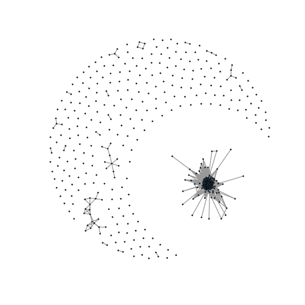
> gno <- delete.isol(g1)
> plot(gno, layout=layout.fruchterman.reingold,vertex.size=1, vertex.label=NA
,edge.width=2)
>
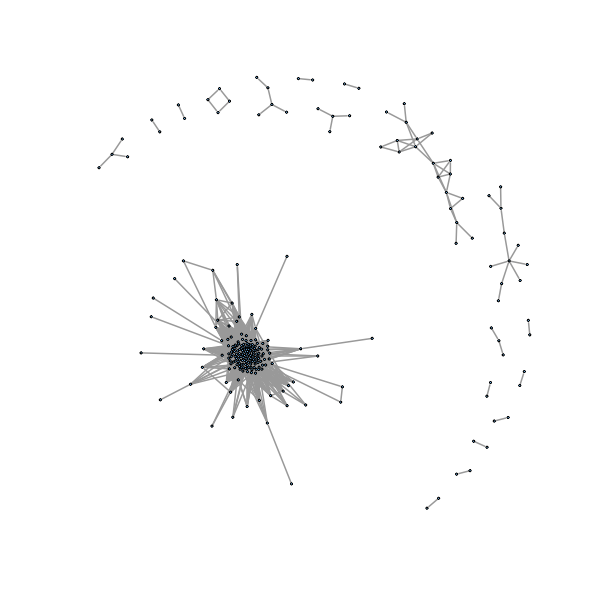
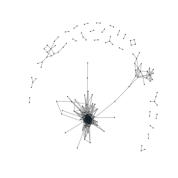
We would like to automatically label connected components, here we want to see what happens if we are a little more loose in defining our threshold so the graph is more connected.
> coinc2=matrix(0,n,n)
> ind2=which((jaacm>0 & jaacm<(1-0.35)),arr.ind=TRUE)
> coinc2[ind2]=1
> g2=graph.adjacency(coinc2,mode="undirected")
> gno2 <- delete.isol(g2)
>
�������������������������������������������������������������������������������������������������������������������������������������������������������������������������������������������������������������������������������������������������������������������������� > plot(gno2, layout=layout.fruchterman.reingold, vertex.size=1, vertex.label= NA, edge.width=2) >
R code for cut and paste
require(igraph)
g1=graph.adjacency(coinc,mode="undirected")
plot(g1, layout=layout.fruchterman.reingold,vertex.size=1, vertex.label=NA,edge.width=2)
delete.isol <- function(graph) {
   isolates <- which(degree(graph, mode = 'all') == 0) - 1
   igraph::delete.vertices(graph, isolates)
   }
gno <- delete.isol(g1)
plot(gno, layout=layout.fruchterman.reingold,vertex.size=1, vertex.label=NA,edge.width=2)
coinc2=matrix(0,n,n)
ind2=which((jaacm>0 & jaacm<(1-0.35)),arr.ind=TRUE)
coinc2[ind2]=1
g2=graph.adjacency(coinc2,mode="undirected")
gno2 <- delete.isol(g2)
plot(gno2, layout=layout.fruchterman.reingold, vertex.size=1, vertex.label=NA, edge.width=2)