|
Research
Sediment transport modelingUsing drones to infer suspended sediment concentrationsFine sediment transport in estuariesIn San Francisco Bay and similar estuaries, sediments are primarily composed of silts and clays, and hence they are cohesive and succeptible to flocculation, wherein fine sediment particles aggregate (or flocculate) to form larger flocs. Flocculation and breakup mechanisms dictate suspended sediment transport in estuaries because the size of the flocs determines their settling velocity, and hence deposition rate. If the turbulence is strong, flocs can be broken up into smaller flocs and are suspended for longer periods in the water column due to slower settling, while weak turbulence encourages flocculation and more rapid settling. Despite the importance of cohesive sediment in estuarine sediment transport, three-dimensional sediment transport models do not incorporate cohesive sediment processes because of a fundamental lack of understanding of how to incorporate flocculation mechanisms into the models.My research group studies sediment transport in San Francisco Bay to understand the physical mechanisms leading to resuspension and transport of cohesive sediments due to the combined action of tidal currents and wind waves. We developed a wave model for SUNTANS to incorporate the effects of wind-waves and the associate wave-driven sediment resuspension in San Francisco Bay (Chou et al., 2015). An added complication of sediment transport in estuaries is that the fine, cohesive sediments form mud layers on the bed which act to damp waves. Therefore, accurate fine sediment modeling requires two-way feedback between waves and sediments, since the thickness of the mud layer plays an essential role in the amount of wave damping (Figure 1).
Despite the importance of cohesive sediments in estuaries, we have found that accurate model predictions of the suspended sediment concentration (SSC) in South San Francisco Bay can be achieved through transport of two size classes in which the sizes remain fixed throughout the simulations. The size classes are given by micro and macroflocs to represent the behavior of two floc sizes; the microflocs represent fine sediments that tend to remain in suspension over time scales that are longer than a tidal cycle, while the macroflocs are resuspended during wave events and settle over shorter time scales. Although flocculation physics are not incorporated, the size classes are referred to as flocs given that they are representative of the observed flocs in the system. In addition to use of two size classes, a key element of reproducing the observed SSC time series is correct specification of the relative contribution of each size class that is eroded from the bed, which we refer to as the micro/macro floc ratio Rm/M. As an example, if Rm/M=0.25, this implies that, when the local stress exceeds the critical stress (of roughly 0.1 Pa), the mass of resuspended microflocs is 25% of the mass of the resuspended macroflocs. We studied the effects of Rm/M on sediment transport in South San Francisco Bay (Chou et al., submitted) and compared the results to observations in the channel and shoals of the bay (Figure 2). Using the model, we found that most of the observed SSC on the shoals arises from local wind-wave resuspension, while that in the channels arises predominantly from resuspension on the shoals and subsequent transport into the channels. As a result of the fundamentally different behavior of the suspensions on the shoals and channels, different values of Rm/M must be used in the main channel and the shallow shoals of the bay to obtain good agreement between model results and observations. Specifically, in the channel, Rm/M=0.05, whereas on the shoals, Rm/M=0.43, reflecting the fact that the shoals are the dominant source of fine sediments in the channels. For predictive modeling it would not be possible to calibrate the micro/macro floc ratio, but instead a bed model that simulates the evolution of Rm/M based on long-term sediment deposition and bed consolidation processes would be needed.
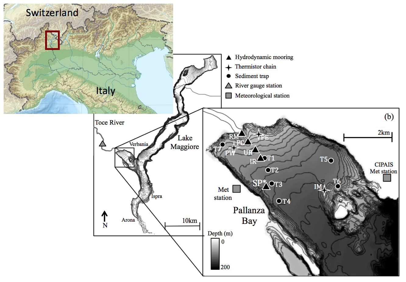
Three-dimensional river plume modelingScheu et al. (2015) and Scheu et al. (submitted) used the SUNTANS model to understand the transport of fine sediment from the Toce River in Lake Maggiore, Italy (Figure 3). Figure 4 presents the evolution of the sediment plume from a typical river inflow event during late summer when the stratification is well developed. Because the river is colder than the surface waters, the plume plunges to a depth of roughly 20 m, where its density matches that of the surrounding waters. Due to the Coriolis effect at this high-latitude lake, the plume turns to the right and follows the southern boundary of Pallanza Bay. The sediments that flow out into the bay are composed primarily of fine silts, and hence they take longer to settle than the time period of the inflow event. Compared to observations, however, the model underpredicts the observed settling rates, which is likely due to a lack of convective settling in the model.
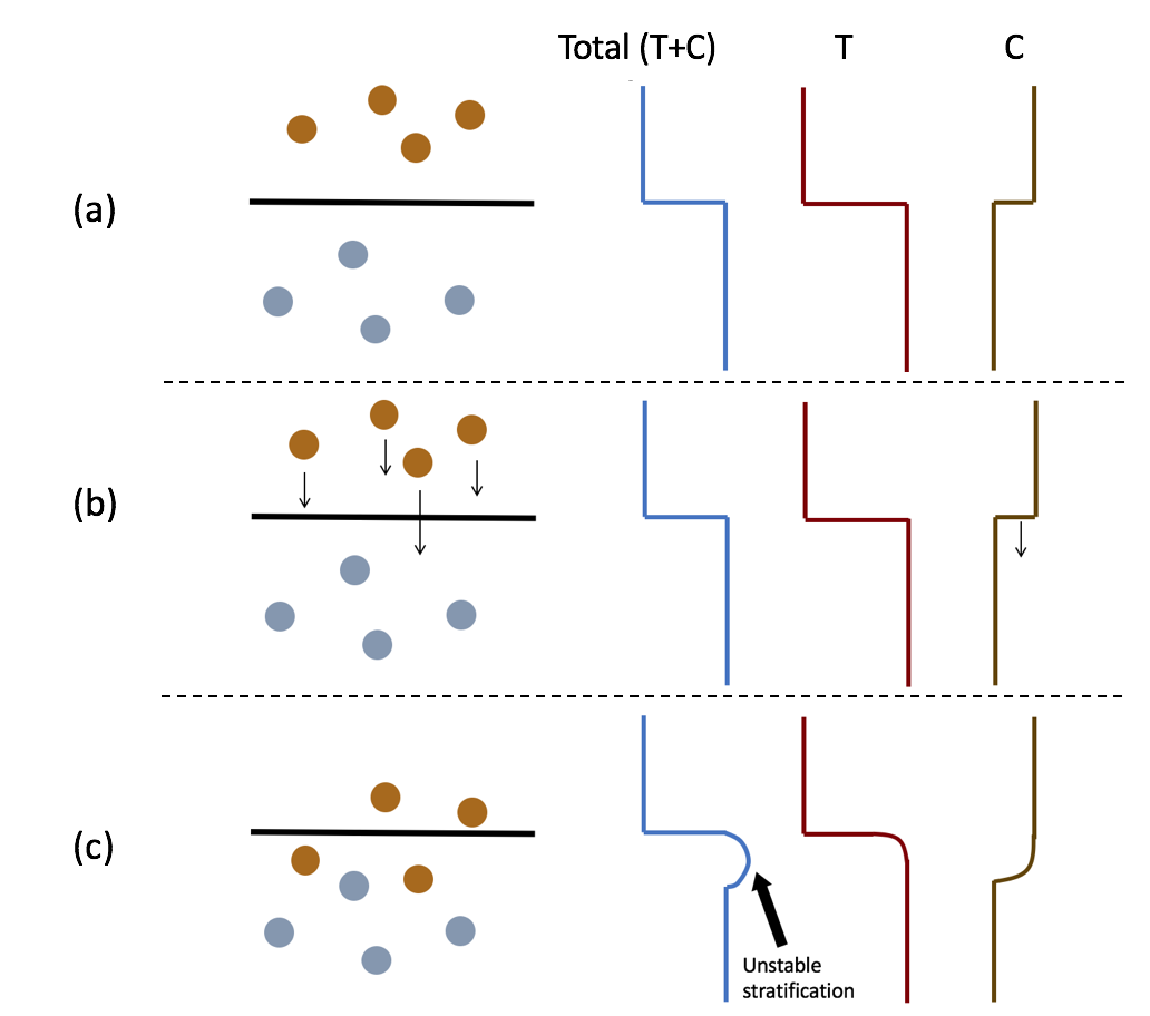
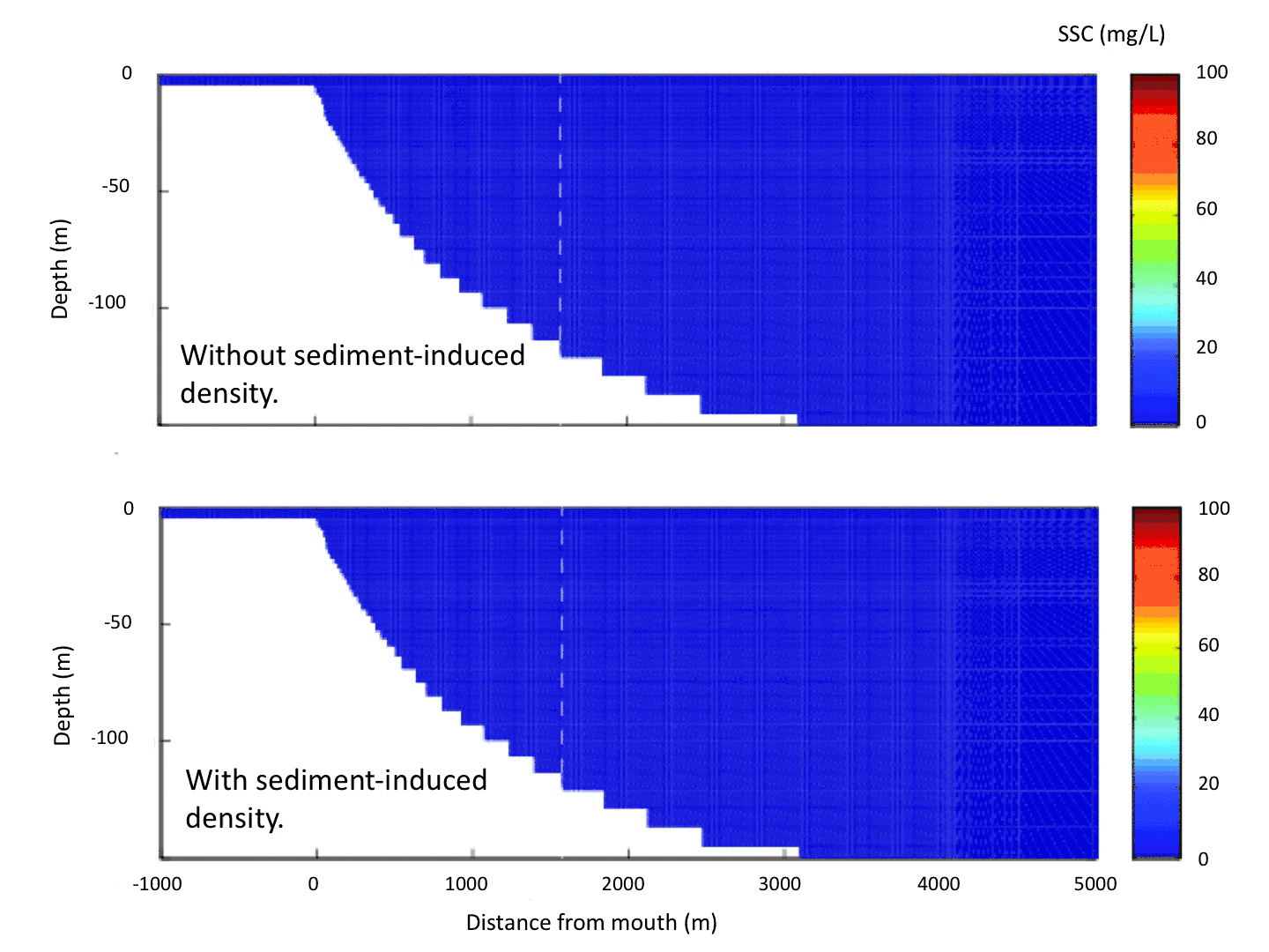
Convectively-driven settlingConvectively-driven settling occurs due to sediment-induced density effects. Although the sediment plume in Figure 4 plunges to a depth of neutral buoyancy and is initially stable, sediment within the plume settles and leads to a statically unstable situation below the plume in which dense, sediment-laden water is more dense than the surrounding waters (Figure 5). This leads to convective instabilities and rapid settling at a rate that is much faster than the Stokes' settling velocity of individual sediment grains. There are no parameterizations that correctly take into account convectively-driven settling of an unstable sediment plume. However, the two-equation turbulence closure scheme in the SUNTANS model (Mellor and Yamada level 2.5 model) takes the unstable stratification into account, to some degree, by predicting a large vertical eddy-diffusity when there is unstable stratification. This gives strong vertical mixing that acts to increase the downward settling flux, although not at the rate expected due to convectively-driven settling.If there are sufficient computational resources, convectively-driven settling can be directly simulated with a horizontal grid resolution that resolves the convective plumes, as shown in Figure 6. The grid resolution needed to simulate convectively-driven settling in the three-dimensional model depicted in Figure 4 would need to be increased by a factor of ten in both horizontal directions (from 40 m to at least 4 m), thus increasing the total number of grid cells in three dimensions from 3 million to 300 million. Since convectively-driven settling is a nonhydrostatic process, the increase in problem size would be accompanied by the need to compute the nonhydrostatic pressure, which also substantially increases the computation time. Although the problem size needed to directly compute convectively-driven settling in the three-dimensional model is tractable on modern supercomputers, the increase in computational cost would not lead to equivalent gains in model ability to compute the correct deposition. Through comparison to sediment traps in Pallanza Bay, Scheu et al. (submitted) showed excellent agreement between modeled and observed depositional patterns without convectively-driven settling in the model. The agreement is likely because much of the settling occurs after the plume, which is driven by an inflow event lasting less than one day, has lost most of its horizontal momentum. Therefore, there is no added model skill in computing the correct settling flux as long as the model does a reasonable job of computing the horizontal transport. Scheu et al. (submitted) show that the horizontal currents, suspended sediment, and temperature are accurately predicted, which explains the good predictions of deposition despite the lack of convectively-driven settling.
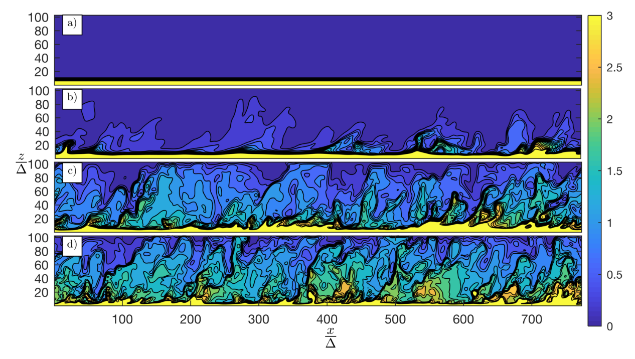
LES of the formation and evolution of sand ripplesMy group developed a large-eddy simulation code to simulate suspended sediment with a moving bed and a rough wall bottom boundary condition (Chou and Fringer, 2008; Chou and Fringer, 2010a; Chou and Fringer, 2010b). This code was used to understand the evolution of the suspension in a rough wall turbulent channel flow (Figure 7) and to understand the formation of sand ripples in response to wave-current turbulence (Figure 8 and Figure 9). When simulating the evolution of ripples, small ripples do not require a model for suspended load since the flow is not energetic enough to suspend the sediment. Therefore, such smaller, rolling-grain ripples only require a bed-load model. However, when the ripples become larger, they are classified as vortex ripples, wherein flow separation over the ripple crests leads to strong turbulence and sediment resuspension. Therefore, vortex ripples require computation of suspended sediment. The model of Chou and Fringer (2010b) accurately computes the formation and evolution of vortex ripples (Figure 8 and Figure 9), although we show that no explicit bed-load model is needed. Instead, strong stratification by the suspension near the bed inhibits turbulence and creates a high-concentration near-bed sediment layer that effectively acts as bed load.
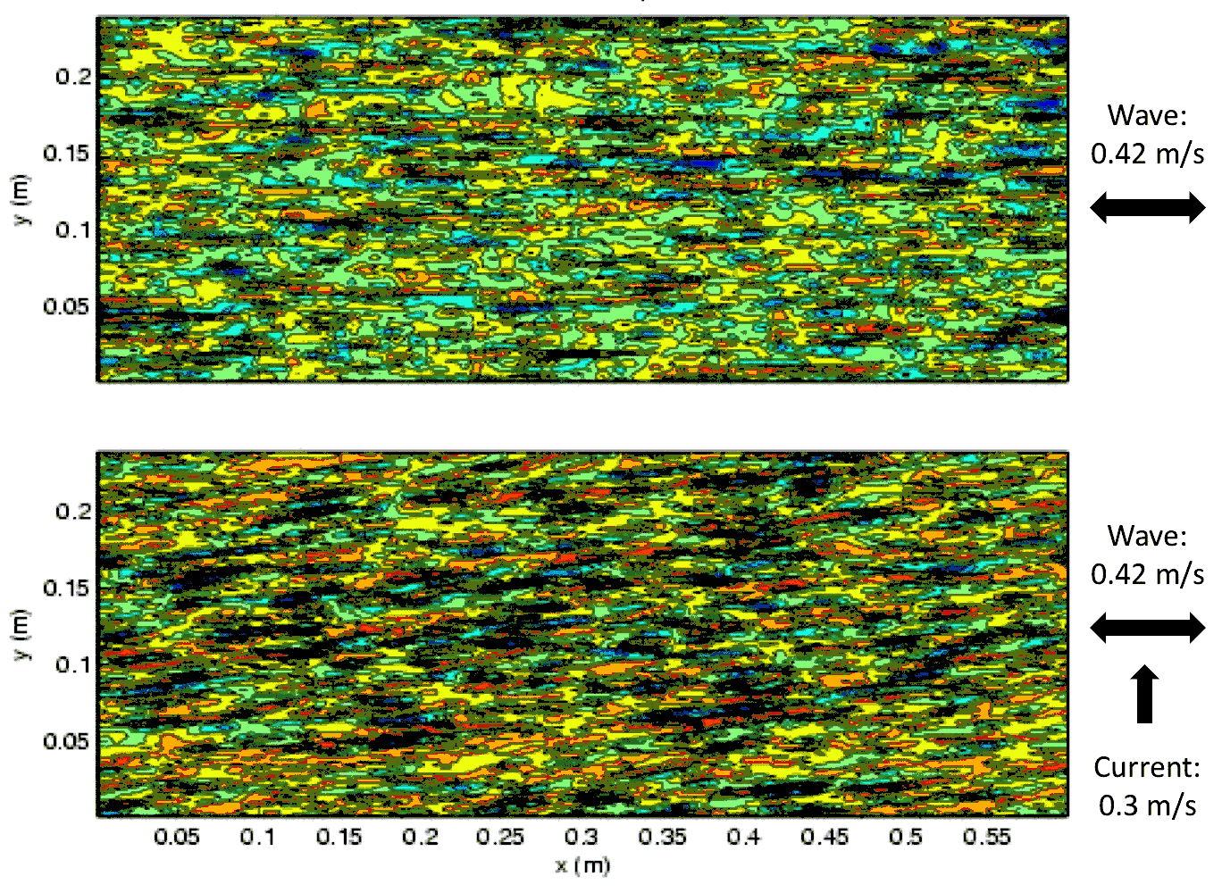
DNS of wave-current suspended sediment dynamicsIn addition to parameterizing the unresolved turbulence, field-scale models must also parameterize the effects of waves and currents on the bottom stress because surface waves are not resolved. Most models take the vector sum of the current and wave-driven bottom stress (the wave-driven bottom stress is computed with the wave amplitude and period which are obtained from the wave model; e.g. Chou et al., 2015) to compute the total wave-current bottom stress, along with adjustments based on turbulent wave-current boundary layer theory, such as that of Grant and Madsen (1979; doi:10.1029/JC084iC04p01797). However, these theories assume a turbulent wave boundary layer over a rough wall, which is valid in nearshore, sandy, wave-driven environments. Therefore, it may not be valid in estuarine environments where the wind-wave field typically drives laminar wave boundary layers over beds that are hydraulically smooth because of the presence of fine sediments typical in estuaries. Using DNS to simulate wave-current boundary layers (Figure 10), we have found the surprising result that the addition of waves can act to reduce the wave-current bottom stress and subsequent sediment erosion. This occurs because the bottom stress is reduced during half of the wave cycle when the wave pressure gradient opposes the mean pressure gradient, thus laminarizing the steady turbulent flow for part of the wave period.
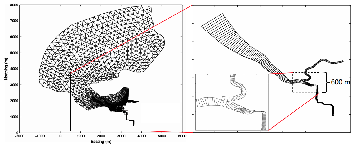
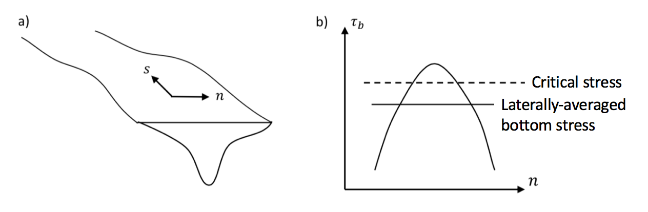
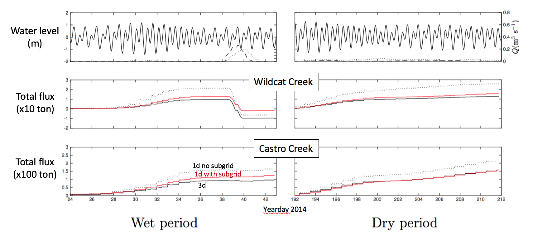
Although the subgrid bathymetry method can correctly reproduce the flow and stage in a compound channel, the bottom stress must be reconstructed to correctly capture the sediment resuspension and transport, since the bottom stress on the coarse hydrodynamic grid would underpredict the erosion and subsequent transport, as shown in Figure 12. We have developed a method to reconstruct the subgrid erosion based on reconstruction of the velocity field and bottom stress by assuming a balance between bottom friction and the barotropic pressure gradient (discussed here). While this is relatively straightforward, it is more difficult to reconstruct the subgrid deposition since it requires knowledge of the subgrid variability of the suspended sediment concentration. We have developed a parameterization that reconstructs the deposition based on the distribution of vegetation in the system, which captures some of the subgrid variability in the suspended sediment since we expect weaker suspensions where there is vegetation. Application of our subgrid method to the salt marsh estuary in the Castro Cove Region shows good agreement between the sediment transport computed with the three-dimensional model and that computed with the one-dimensional model using subgrid bathymetry (Figure 13).
|
|||
| Last updated: 09/26/25 | ||||