|
Research
Numerical model developmentA unique feature of my research group is that we focus on development and implementation of numerical models over scales ranging from those related to fine-scale turbulence physics and mixing to those at large scales related to coastal circulation and transport. Numerical modeling of these processes requires fundamentally different approaches. The fine scale processes are simulated with computer codes that directly discretize the Navier-Stokes equation with little to no approximations, including the large-eddy simulation (LES) and direction numerical simulation (DNS) approaches. The large-scale processes, on the other hand, are simulated using ocean models that discretize simplified or approximate forms of the Navier-Stokes equation, such as the hydrostatic approximation. In these models, because the turbulence is not resolved, they employ the Reynolds-averaged form of the Navier-Stokes equation in the so-called RANS approach, wherein the turbulence is parameterized. In addition to the errors arising from the approximate forms of the equations, a fundamentally different aspect of large-scale circulation modeling is that many of the errors arise from a lack of knowledge of boundary and initial conditions (e.g. bottom bathymetry, wind fields for surface stresses, initial temperature and salinity fields, etc…). Therefore, a key element of the research in my group related to ocean modeling is balancing the cost related to more accurate representation of the physics with improved numerical modeling techniques against the intrinsic errors related to boundary and initial conditions. Given that Navier-Stokes solvers employ few approximations, a long-term goal of ours is to develop ocean models that employ techniques often restricted to Navier-Stokes solvers.
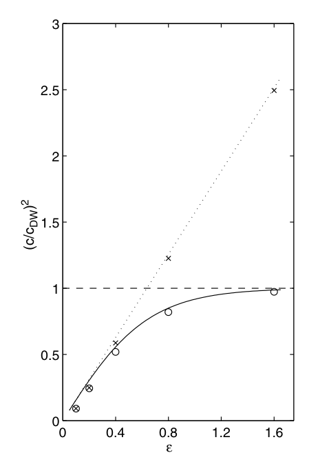
The most straightforward test of a nonhydrostatic model is a standing wave in a tank. Since my research group focuses on internal gravity waves, we focus on testing nonhydrostatic effects in an internal seiche, as shown in Figure 1. Application of a nonhydrostatic model to simulate the oscillations will correctly reproduce the dispersive wave speed as the domain is made deeper. As shown in Figure 2, in the limit of water very deep relative to the wavelength, the wave speed approaches the deep-water wave speed because it depends on the length of the tank (which is half the wavelength) and not the depth when D≫L. However, use of a hydrostatic model implies that the speed is only a function of the depth, and so the wave speed continues to increase with increasing tank depth.
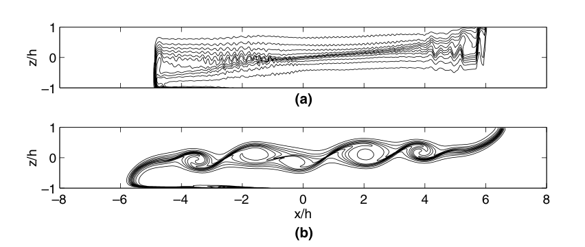
Another excellent example of a strongly nonhydrostatic process is the nonhydrostatic lock exchange problem, as shown in Figure 3. In this problem, a tank is filled with two fluids of different densities separated by a “lock”. Releasing the lock creates an exchange flow with shear instabilities at the interface. Because these instabilities are characterized by vertical and horizontal length scales that match, their aspect ratio is unity, implying that they cannot be reproduced by a hydrostatic model.
Calculation of nonhydrostatic processes is computationally expensive because of the need to employ high grid resolution to resolve processes with short horizontal length scales. It is also expensive because solution of the nonhydrostatic pressure involves inversion of a large, linear system of equations, which can increase the computational cost of an ocean model by up to one order of magnitude. Fortunately, however, in Fringer et al. (2006), we show that if suitable preconditioners are employed when inverting this linear system, the cost of computing the nonhydrostatic pressure vanishes when the leptic ratio, or lambda=dx/D (Scotti and Mitran, Ocean Modeling, 2008), is large. That is, if the grid resolution dx is large relative to the depth D, then nonhydrostatic effects are not being resolved, and so inclusion of the nonhydrostatic pressure does not incur computational overhead. This is useful for unstructured-grid models in which the grid resolution is refined in regions where nonhydrostatic effects are important, but coarse where it is not. The resulting solver thus only needs to do work in regions where the lepticity is small, or where the nonhydrostatic effects are important, and there is no overhead related to computation of the nonhydrostatic pressure. Although nonhydrostatic models are expensive because they require high grid resolution, it is useful to understand the minimum grid resolution needed to resolve the nonhydrostatic effect of interest. My research group works extensively on nonhydrostatic simulations of internal gravity waves, and we have developed a criterion dictating the grid resolution needed to resolve the leading-order nonhydrostatic effect in such waves. Many large-scale simulations of internal waves are computed with ocean models solving the primitive (hydrostatic) equations. Weakly nonlinear internal waves, however, represent a dynamical balance between nonlinearity and nonhydrostasy (dispersion), and thus may require more computationally expensive nonhydrostatic simulations to be well-resolved. Most discretizations of the primitive equations are second-order accurate, inducing numerical dispersion generated from odd-order terms in the truncation error (3rd-order derivatives and higher). This numerical dispersion mimics physical dispersion due to nonhydrostasy. In the analysis detailed in Vitousek and Fringer (2011), we determine the numerical dispersion coefficient associated with common discretizations of the primitive equations. Comparing this coefficient with the physical dispersion coefficient from the Boussinesq wave equations, we find that, to lowest order, the ratio of numerical to physical dispersion is Gamma = K lambda^2 where K is an O(1) constant dependent on the discretization of the governing equations and the grid leptic ratio is defined as lambda = dx/h1, where dx is the horizontal grid spacing and h1 is the depth of the internal interface. Typical scales in the ocean are very long relative to their depth and hence extraordinarily thin. Likewise, typical grid resolutions in ocean models reflect these thin scales, resulting in large values of lambda. Thus, simulations may be overly (numerically) dispersive as dictated by the relationship Gamma = K lambda^2. When the grid lepticity is large, solitary wave widths of hydrostatic and nonhydrostatic models converge to each other due to the overwhelming presence of numerical dispersion. An illustration of this effect is given in Figure 4. In this example, nonhydrostatic and hydrostatic models provide practically identical results, which gives a false impression that nonhydrostatic effects must therefore be unimportant. Using a much smaller lepticity, the physical nonhydrostatic dispersion is resolved, producing the correct waves as shown in Figure 5. In this case, however, since the numerical dispersion in the hydrostatic model is so small, short, "numerical solitons" are created in the hydrostatic model. These are susceptible to numerical diffusion which causes amplitude loss and a reduction in amplitude dispersion, thereby creating a slower wave.
The nonhydrostatic grid-resolution criterion poses significant computational challenges for resolving nonhydrostatic internal gravity waves in the ocean. An example calculation of internal gravity waves is shown in Figure 6, which depicts an animation of the elevation of the 20 degree isotherm in the South China Sea due to internal wave generation by tidal flow over steep bathymetry between Taiwan and Luzon, Phillippines. As described in Zhang et al. (2011), the simulation required 12 million grid cells and hundreds of thousands of CPU hours (a lot in 2007!) to simulate two weeks of real time (one spring-neap tidal cycle). Despite the computational expense, those simulations employed a grid resolution that was dx=1000 m with a mixed-layer depth of h1=200 m, implying a large leptic ratio (lambda=dx/h1=5) and hence lack of resolution of the leading-order nonhydrostatic processes related to the internal solitary waves. If we were to employ a grid resolution with lambda=0.5, this would require an increase in the computational expense by roughly a factor of at least 50, or 1.2 billion grid cells.
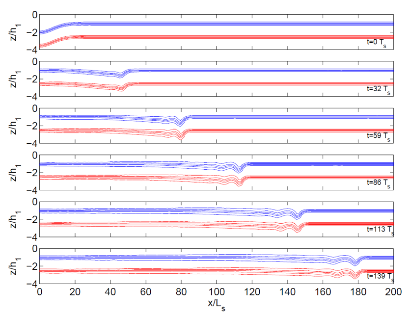
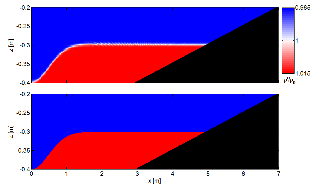
To alleviate the computational expense related to resolution of leading-order nonhydrostatic effects in internal gravity waves, my research group (Vitousek and Fringer, 2014) developed a nonhydrostatic, isopycnal-coordinate ocean model that employs a vertical grid that follows the lines of constant density (isopycnals), using the arbitrary Lagrangian-Eulerian (ALE) framework commonly employed in Navier-Stokes solvers with moving grids (e.g. Koltakov and Fringer, 2013). Although isopycnal coordinates are common in ocean modeling, ours is the first nonhydrostatic model. The advantage of isopycnal coordinates is that nonphysical numerical diffusion is eliminated because, by definition, there is no transport of density across grid lines. Therefore, the number of grid cells needed to resolve the vertical dimension can be reduced by an order of magnitude, thus reducing the computational expense of the problem. Isopycnal coordinates can have problems when physical vertical mixing is desired – to accommodate this effect we have also developed a hybrid-coordinate, nonhydrostatic model, wherein the vertical coordinate is arbitrary so it can accommodate vertical mixing if desired. An example of a result with the nonhydrostatic, isopycnal-coordinate model of Vitousek and Fringer (2014) is shown in Figure 7, which shows the evolution of internal tides as they steepen into trains of internal solitary-like waves. This result was obtained with just 10 isopycnal layers as opposed to 100 z-levels, which would be required with a traditional z-level model, thus representing a cost savings of a factor of ten. Surprisingly, just a few layers are needed to reproduce complex physics. For example, Figure 8 compares the result of a breaking internal gravity wave on a slope using the isopycnal-coordinate model of Vitousek and Fringer (2014) to a three-dimensional, large-eddy simulation (LES) result of Arthur and Fringer (2014). The breaking dynamics are very similar despite the use of just two isopycnal layers with no model to parameterize the cross-isopycnal flux due to mixing.
Not only are quadrilaterals ideally suited to resolving long channels, but our research has shown that they alleviate grid-scale noise that is common in unstructured, triangular grids in which the pressure is defined at the cell centers and the velocity is defined normal to the cell edges (Wolfram and Fringer, 2013). Such an arrangement is useful for accurate solutions of the linear shallow water equations, although only the normal component of velocity is typically stored at the cell faces. Therefore, special care must be taken for nonlinear problems that require more accurate reconstruction of the component of flow tangent to the cell faces (Wang et al., 2011). My research group continuously works to add to the features of the SUNTANS model (Fringer et al., 2006) to improve its functionality in different environments. These include the development of a sediment transport model (Chou et al., submitted) and a spectral wave model to include the effects of wave-driven currents and bottom stresses (Chou et al., 2015). We have also implemented the cut-cell approach that enables use of a Cartesian grid in the vertical that follows variable bottom geometry smoothly rather than with stair-stepping. To simulate flows in salt-marsh estuaries, we have implemented a marsh vegetation drag module along with a culvert module. Finally, the SUNTANS code now incorporates the method of subgrid bathymetry, whereby bathymetry data at a resolution that is finer than the mesh are incorporated into the solution without increasing the resolution of the underlying computational mesh. These features are under development.
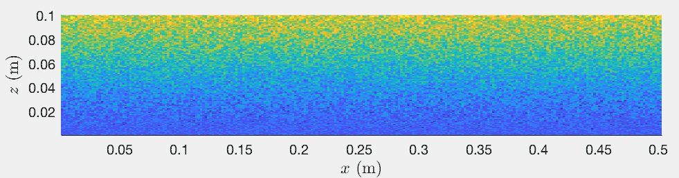
The Navier-Stokes codes with which my group works employ resolution that is sufficient to resolve the turbulent dynamics of the flow field. We employ both the large-eddy simulation (LES) and Direct Numerical Simulation (DNS) approaches. In LES, most of the turbulence is resolved and the unresolved turbulence is accounted for with turbulence models, while in DNS all of the turbulence is resolved. For example, Chou and Fringer (2008) developed an LES model for the simulation of suspended sediment in a rough-wall channel flow, while Arthur and Fringer (2014) and Arthur et al. (2017) performed DNS of a breaking internal wave on a slope. Much of our sediment work involves simulation of turbulent channel flow which requires countless computational hours for the flow to reach turbulent equilibrium (Figure 13). To alleviate this expense, we developed a procedure that reduces the spin-up time by nearly one order of magnitude, as outlined in Nelson and Fringer (2017). The method provides savings worth hundreds of thousands of CPU hours in high-resolution simulations of turbulent channel flow.
|
|||
| Last updated: 09/26/25 | ||||