|
home
people
research
publications
scholar
SUNTANS
krell fellowships
|
 |
|
Research
Internal waves
Internal bores
Much like surface gravity waves, internal gravity waves steepen, break
and lead to mixing and transport in lakes and coastal oceans. My group
works extensively on modeling and understanding of
high-frequency, nonlinear waves and bores that are often observed in
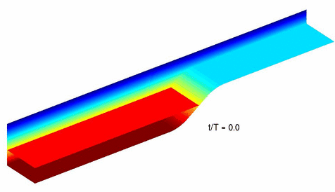
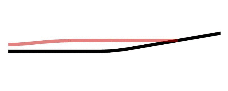
shallow (<50 m) continental shelf waters. A simulation of an internal bore, or
bolus, that is generated by the interaction of an internal wave with a shelf break,
is depicted in Figure 1.
Figure 1: Generation of an internal bore, or bolus, due to the interaction of
an internal gravity wave with a shelf break. Here, T is the wave period. (From Venayagamoorthy and Fringer, 2007).
An interesting feature of
nonlinear internal waves in coastal waters is that they exhibit differing behavior
depending on the Iribarren number, which is a ratio of topographic slope
to a measure of the internal wave steepness. This behavior was demonstrated
with the SUNTANS model to understand observations of interal bore-driven
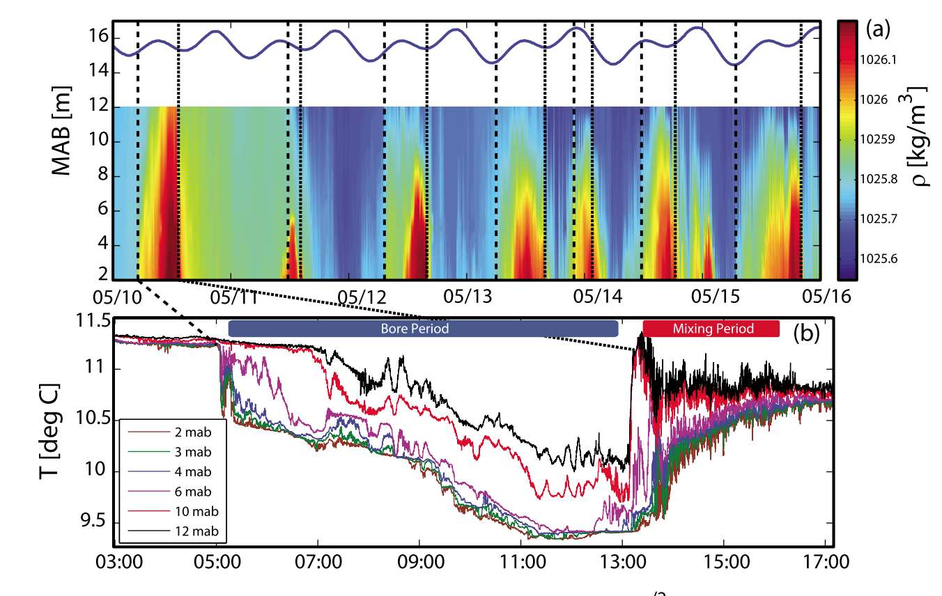
turbulence in shallow waters of Monterey Bay, CA. Observations of Walter et al. (2012) depicted in
Figure 2 show time series of the gradual arrival of a bore followed by an abrupt transition to
turbulence. This behavior is not what is typically expected of a bore time series in coastal
waters, since we expect the canonical behavior in which a bore time series
features a strong, leading edge or shock, followed by
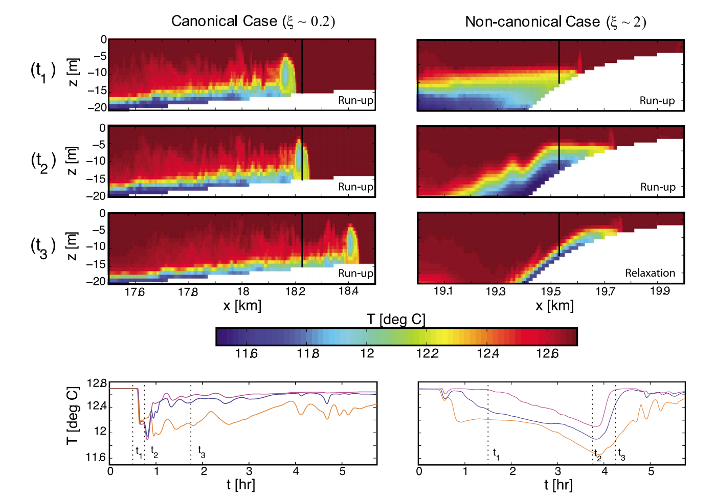
a smooth relaxation associated with its tail. Simulations with the SUNTANS model
(Figure 3) show that such canonical behavior occurs for gradual slopes relative to the internal wave slope,
or small Iribarren numbers, while the noncanonical behavior indicated by the time series
in Figure 2 arises for steeper slopes, or larger Iribarren numbers.
Figure 2: Observed density contours in 15 m of water in Monterey Bay (a), showing the
arrival of dense, cold-water bores. The zoomed-in view of a particular event in (b)
shows the noncanonical behavior of the bores in which a gradual arrival (the bore period)
is followed by an abrupt transition to the mixing period. The blue line in (a) is the
free surface, while each line in (b) represents data from a thermistor at the indicated
depth in mab (meters above bottom). (From Walter et al., 2012).
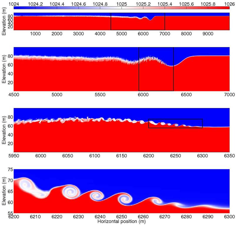
Figure 3: SUNTANS simulations of temperature signals of internal bores
for a canonical case with an Iribarren number of 0.2 (left panels) and a noncanonical case
with an Iribarren number of 2 (right panels). The top three rows represent the temperature
field at the points in time indicated in the bottom time series, which show temperature
time series at 2, 4, and 6 mab (meters above bottom). The time series are taken from
a point in the domain where the water is 15 m deep, indicated by the vertical black line in the top
panels. The noncanonical case is similar to the observations in Figure 2. (From
Walter et al., 2012).
Trapped internal Kelvin waves
|
back to top
|
Although internal bores in the ocean are typically generated by
shoaling internal tides, or internal waves of tidal frequency,
propagating normal to a coastline, they can also arise due to
trapped nonlinear internal Kelvin waves propagating parallel to the coastline.
Internal waves can be trapped when their frequency is less than the local inertial frequency,
in which case they exist as trapped Kelvin waves rather than freely propagating
internal waves.
Temperature time series in 15 m of water on the southern side of
Oshima Island in Japan (Figure 4) show strong diurnal motions that arise
because the frequency of the internal Kelvin wave (which is trapped) that propagates around
the island matches the diurnal tidal frequency, thus producing resonance.
The trapped internal Kelvin waves are visible in the animations in Figure 5, which shows how the
diurnal internal waves propagate along the coastlines while the semidiurnal internal waves
freely propagate. Figure 6 shows energy flux associated with internal waves that
arise with semidiurnal and diurnal forcing. Owing to resonance of
the internal Kelvin waves (around many of the islands in the region), the
diurnal energy flux is significantly stronger than the semidiurnal
energy flux.
Figure 4: Observed (top) and modeled (bottom)
temperature times series in shallow water offshore of Oshima Island, Japan, showing
the arrival of cold-water internal bores. These results have been low-pass filtered to eliminate
motions with periods shorter than 3 hours. The bores are predominantly semidiurnal during
the first 7 days, but as the diurnal tides become stronger later in the time series, strong
diurnal internal bores appear. These are signatures of resonant Kelvin waves propagating
around the island. (From Masunaga et al., 2017).
Figure 5: Displacement of the 20C isotherm (at an average depth of 100 m) in response
to barotropic forcing at the diurnal (K1) frequency (left) and the semidiurnal (M2) frequency (right)
around Oshima Island, Japan (in the center of the panels).
Because the local inertial frequency exceeds the diurnal frequency, the K1 waves are trapped and
propagate in a clockwise sense around the islands, while the M2 waves are freely propagating.
(From Masunaga et al., 2017).
Figure 6: Baroclinic energy flux around Oshima Island, Japan (in the center of the panels)
obtained from SUNTANS model results, showing how the diurnal energy flux (a) is roughly
ten times larger than the semidiurnal energy flux (b) due to diurnal internal Kelvin wave
resonance around the island. The energy flux is given by the depth-integrated product
of the pressure and velocity (pu) associated with internal waves, averaged over a
wave period. (From Masunaga et al., 2017).
Breaking and mixing
|
back to top
|
Although the studies that involve the SUNTANS model employ sufficient resolution
to resolve the
leading-order nonhydrostatic effects, the resolution in those studies is
insufficient to resolve the breaking and mixing dynamics. To study such processes, we
employ our Navier-Stokes codes
to perform direct numerical simulations (DNS) of breaking internal
waves. The DNS approach has the advantage that the turbulence and mixing are resolved,
and so do not need to be parameterized.
It is thought that breaking internal waves account for a large fraction of the mixing
driven by the tides in the ocean. However, models that simulate large-scale tidal
processes cannot resolve the mixing driven by the internal waves, and thus those
processes need to be parameterized. A common method to parameterize the mixing is through use of the mixing efficiency,
which is the fraction of wave energy that is lost that is converted into mixing
during breaking. The mixing efficiency is useful for parameterizing
mixing because it enables approximation of the mixing if the dissipation, which is
much easier to measure or model, is known. Based on many measurements of mixing in the ocean, the
average, or canonical, value of the mixing efficiency is 0.17. However, it is hypothesized that
the mixing efficiency can be much higher in the presence of breaking internal waves, and much lower
particularly near boundaries.
My group employs DNS to study the turbulence and mixing
arising from breaking internal waves. Figure 7 shows an
example of an internal wave breaking away from boundaries, while Figure 8 shows an internal wave
breaking on a slope. For these simulations, we compute the bulk mixing efficiency,
which is a ratio of the total energy lost to mixing to the total energy lost
(the sum of dissipation and mixing) during the breaking event, integrated over the domain and
over time. In a series of simulations with different stratifications,
the average bulk mixing efficiency for the periodic wave away from boundaries is 0.42 (Fringer and Street, 2003)
while that for the wave on the slope is 0.31 (Arthur et al., 2017), the lower value
reflecting inefficient boundary-driven mixing.
These values are much higher than the canonical value of 0.17 because they represent
special cases in which the nondimensional pycnocline thickness (k delta) is approximately 1
(k=2pi/lambda is the wavenumber, lambda is the wave length, and delta is the
pycnocline thickness). In such cases, relatively short waves can generate strong convectively-driven
mixing which is very efficient and can have a mixing efficiency as large as 0.5. These waves
are representative of small-scale breaking internal wave events in the ocean and highlight
how the efficiency can be quite high due to breaking internal waves. Simulations of breaking internal
waves with smaller nondimensional pycnocline thicknesses produce mixing efficiencies closer to
the canonical value of 0.17, consistent with shear-driven turbulence which occurs
during breaking in the presence of a relatively thin pycnocline.
Figure 7: Isosurfaces of mean density in a breaking periodic internal wave in deep water (i.e. no bottom
effects). Note how the average wave amplitude decreases substantially after breaking. (From Fringer and Street, 2003).
Figure 8: Isosurface of mean density (red) along with positive and negative vorticity that is
five times the wave frequency (green and blue) of a breaking internal wave on a slope.
(From Arthur and Fringer, 2014).
An important component of mixing parameterizations in addition to the mixing efficiency
is a measure of the local stratification against which the turbulence is
working to mix the fluid. In a recent paper (Arthur et al., 2017), we showed that defining the local
stratification is not obvious, particularly in the presence of a
highly turbulent flow field arising in a breaking internal wave. DNS results indicate that the mixing
parameterization can be off by over an order of magnitude depending on
how the local stratification is defined.
Shear Instabilities
|
back to top
|
As mentioned above, turbulence during breaking becomes primarily
shear-driven when the pycnocline thickness in the internal wave is small. Such shear-driven
turbulence is the product of a shear instability in the waves and
is quantified by the gradient Richardson number, Ri, which is a ratio of the stabilizing
effects of stratifiation to the destabilizing effects of shear. In a steady,
stratified shear layer, instability arises when Ri<0.25, resulting in the formation
of Kelvin-Helmholtz billows. However, such may not
be the case in the highly unsteady stratified flow within a propagating internal wave.
To determine the critical Richardson number in an internal wave,
my group (Barad and Fringer, 2010) performed simulations of field-scale, internal solitary waves
using an adaptive mesh refinement (AMR) code that
enabled resolution of meter-scale Kelvin-Helmholtz billows in a 10-km
long domain (Figure 9). Our simulations indicate that instability occurs
when the critical Richardson number drops below the canonical value of 0.25 for sufficiently long
enough, i.e. when the wave period is much longer than the growth time scale of the instability.
The result is a critical Richardson number for instability of 0.1, much lower than the
canonical value of 0.25.
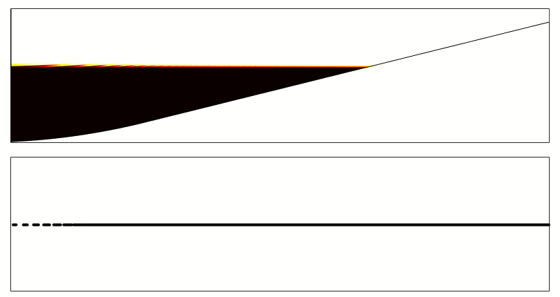
Figure 9: A shear instability arising in a breaking internal solitary wave computed with
an adaptive mesh refinement (AMR) code that allows resolution of meter-scale features in a
domain that is 10 km long. Each panel represents a zoomed-in view of the box shown in
the previous panel. (From Barad and Fringer, 2010).
Transport and dispersion: Breaking waves on slopes
|
back to top
|
In addition to mixing, internal gravity waves are an important contributor to transport
of heat, salt, sediments, nutrients, and biology in coastal environments. To study
mass transport by breaking internal gravity waves on slopes, Arthur and Fringer (2016)
employed the DNS simulations mentioned above along with a particle tracking code.
Simulation results in Figure 10 show how the breaking event leads to transport of particles
both on- and off-shore. This off-shore transport is a likely mechanism explaining
the formation of intermediate nepheloid layers, or layers of turbid fluid found near the
pycnocline in coastal waters.
Figure 10: Simulation of particle transport by a breaking internal gravity wave on a
slope, showing the formation of the intermediate nepheloid layer that propagates offshore
along the pycnocline (the red line). (From Arthur and Fringer, 2016).
Arthur and Fringer (2016) also showed that the cross-shore transport in breaking
internal waves on slopes is accompanied by along-shore dispersion
arising from the turbulence during breaking, as shown in Figure 11. Interestingly,
the along-shore turbulent dispersion exactly matches the turbulent diffusivity expected
from standard two-equation Reynolds-averaged turbulence closure schemes.
Figure 11: Side view of the density field (top panel) and top view of the particles (bottom panel)
during a breaking internal wave on a slope, showing how the breaking leads to strong
along-shore dispersion, as indicated by the alongshore spreading of the particles in the top view.
The red line indicates the plume boundary (three standard deviations of
particles in each of the 100 cross-shore bins), and shows both strong dispersion in the region
of breaking as well as weak spreading (roughly by a factor of 10) away from the breaking region
due to molecular diffusion, represented here by a random walk. (From Arthur and Fringer, 2016).
Transport and dispersion: Internal solitary waves
Internal wave-driven transport and dispersion also occur in internal gravity
waves away from boundaries. If the amplitude of the internal solitary wave
is large enough, it can possess a trapped core of recirculating fluid which
has the potential to transport mass over distances much greater than waves without trapped cores.
Figure 12 shows the dispersion of a point release of particles due to
the passage of an internal solitary wave with and without a trapped core. As described in Gil and Fringer (submitted),
we compute the particle trajectories with the
velocity field obtained with a fully nonlinear form of the stratified Euler equation (the DJL equation),
in addition to a random walk to model local turbulent diffusivity. For waves without trapped
cores, the dominant effect is shear-flow dispersion, whereas transport is dominant for trapped cores.
For waves without trapped cores, shear-flow dispersion leads to
strong horizontal spreading of the particle cloud, although the precise mechanism varies with
the internal wave Peclet number, which is defined as a ratio of the wave advection time scale to
the vertical turbulent diffusive time scale. When the two time scales are roughly equal (Pe~1),
the shear-flow dispersion is maximized. For smaller Peclet numbers (relatively short vertical turbulent diffusion
time scale), the shear flow dispersion is inversely proportional to the vertical turbulent diffusivity,
which is similar to the behavior of longitudinal dispersion in pipes derived by Taylor in 1953.
For large Peclet numbers (relatively long vertical turbulent diffusion time scale), the shear-flow
dispersion is proportional to the vertical turbulent diffusivity, a result that is similar to
longitudinal dispersion in unbounded fluids, such as in atmospheric boundary layers (Saffman, 1962).
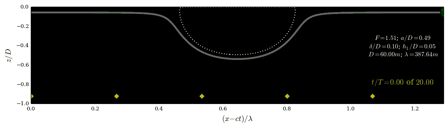
Figure 12: Evolution of a point release of particles during passage of an internal solitary wave
without (top) and with (bottom) a trapped core. Green particles are entrained into the core,
while red particles are not. The pycnocline is indicated by the solid line, while the dotted
line indicates the boundary of the trapped core which is determined by the largest recirculating
streamline. For the parameters indicated in the figures,
F=max(flow velocity)/wave speed is the Froude number, D is the depth, a is the wave amplitude,
delta is the pycnocline thickness, and lambda is the wavelength. (From Gil and Fringer, submitted).
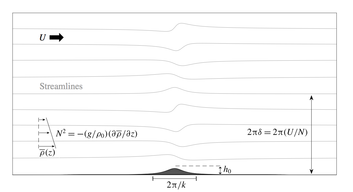
We have recently begun work on internal lee waves, or internal waves
generated by steady, stratified flow over deep-ocean topography, with
an emphasis on parameterizing the drag due to internal lee waves for
large-scale ocean circulation models. As shown in Figure 13, the lee-wave
problem is defined by four parameters, namely the flow speed U, the
stratification N, the topographic height h0, and the topographic length
L=2 pi/k. The ocean depth, D, is not a parameter because we consider flow speeds U
that are much smaller than the mode-1 internal wave speed, c1=N D/pi,
thus implying an infinitely large Froude number defined by Fr=U/c1.
The four parameters can be combined to give the nondimensional
parameters epsilon=U k/N and J=N h0/U. The first parameter is the nonhydrostatic
parameter and is a measure of the vertical scale of the perturbation (U/N) to the
length of the topography (1/k), and typically epsilon ≫ 1 since most flows of
interest are long relative to their vertical scale, and hence hydrostatic.
The second parameter, J, has lacked a unified interpretation for more than 50 years
in the literature and has been referred to by many names,
including the Russel Number, blocking parameter, inverse Froude number,
and vertical Froude number. By studying the linearized Euler equations with stratification,
we show in Mayer and Fringer (2017) that J scales identically with a ratio of the vertical flow velocity to
the vertical group velocity, and hence it should be interpreted as a lee-wave Froude number.
Such an interpretation holds for linear flows up until J=1, beyond which J instead informs the
degree of blocking of the topography. That is, for strong stratification and/or tall topography,
the flow lacks the kinetic energy needed to flow over the hill and is blocked.
Figure 13: Sketch of the lee wave problem, showing the flow speed U, the stratification N,
the topographic length 2 pi/k, the vertical scale delta=U/N, and the topographic height h0. The streamlines represent
flow for the case epsilon=U k/N=0.01 and J=N h0/U=0.5. (From Mayer and Fringer, 2017).
|
|
|
Last updated:
09/26/25
|