Chapter 4
Learning in PDP Models: The Pattern Associator

In previous chapters we have seen how PDP models can be used as content-addressable memories and constraint-satisfaction mechanisms. PDP models are also of interest because of their learning capabilities. They learn, naturally and incrementally, in the course of processing. In this chapter, we will begin to explore learning in PDP models. We will consider two “classical” procedures for learning: the so-called Hebbian, or correlational learning rule, described by Hebb (1949) and before him by William James (1950), and the error-correcting or “delta” learning rule, as studied in slightly different forms by Widrow and Hoff (1960) and by Rosenblatt (1959).

We will also explore the characteristics of one of the most basic network architectures that has been widely used in distributed memory modeling with the Hebb rule and the delta rule. This is the pattern associator. The pattern associator has a set of input units connected to a set of output units by a single layer of modifiable connections that are suitable for training with the Hebb rule and the delta rule. Models of this type have been extensively studied by James Anderson (see Anderson, 1983), Kohonen (1977), and many others; a number of the papers in the Hinton and Anderson (1981) volume describe models of this type. The models of past-tense learning and of case-role assignment in PDP:18 and PDP:19 are pattern associators trained with the delta rule. An analysis of the delta rule in pattern associator models is described in PDP:11.

As these works point out, one-layer pattern associators have several suggestive properties that have made them attractive as models of learning and memory. They can learn to act as content-addressable memories; they generalize the responses they make to novel inputs that are similar to the inputs that they have been trained on; they learn to extract the prototype of a set of repeated experiences in ways that are very similar to the concept learning characteristics seen in human cognitive processes; and they degrade gracefully with damage and noise. In this chapter our aim is to help you develop a basic understanding of the characteristics of these simple parallel networks. However, it must be noted that these kinds of networks have limitations. In the next chapter we will examine these limitations and consider learning procedures that allow the same positive characteristics of pattern associators to manifest themselves in networks and overcome one important class of limitations.

We begin this chapter by presenting a basic description of the learning rules and how they work in training connections coming into a single unit. We will then apply them to learning in the pattern associator.

4.1 BACKGROUND

4.1.1 The Hebb Rule

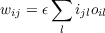
In Hebb’s own formulation, this learning rule was described eloquently but only in words. He proposed that when one neuron participates in firing another, the strength of the connection from the first to the second should be increased. This has often been simplified to ‘cells that fire together wire together’, and this in turn has often been representated mathematically as:

(4.1)

Here we use ϵ to refer to the value of the learning rate parameter. This version has been used extensively in the early work of James Anderson (e.g., Anderson, 1977). If we start from all-zero weights, then expose the network to a sequence of learning events indexed by l, the value of any weight at the end of a series of learning events will be

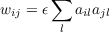(4.2)

In studying this rule, we will assume that activations are distributed around 0 and that the units in the network have activations that can be set in either of two ways: They may be clamped to particular values by external inputs or they may be determined by inputs via their connections to other units in the network. In the latter case, we will initially focus on the case where the units are completely linear; that is, on the case in which the activation and the output of the unit are simply set equal to the net input:

(4.3)

In this formulation, with the activations distributed around 0, the w_ij assigned by Equation 4.2 will be proportional to the correlation between the activations of units i and j; normalizations can be used to preserve this correlational property when units have mean activations that vary from 0.

The correlational character of the Hebbian learning rule is at once the strength of the procedure and its weakness. It is a strength because these correlations can sometimes produce useful associative learning; that is, particular units, when active, will tend to excite other units whose activations have been correlated with them in the past. It can be a weakness, though, since correlations between unit activations often are not sufficient to allow a network to learn even very simple associations between patterns of activation.

First let’s examine a positive case: a simple network consisting of two input units and one output unit (Figure 4.1A). Suppose that we arrange things so that by means of inputs external to this network we are able to impose patterns of activation on these units, and suppose that we use the Hebb rule (Equation 4.1 above) to train the connections from the two input units to the output unit. Suppose further that we use the four patterns shown in Figure 4.1B; that is, we present each pattern, forcing the units to the correct activation, then we adjust the strengths of the connections between the units. According to Equation 4.1, w₂₀ (the weight on the connection to unit 2 from unit 0) will be increased in strength for each pattern by amount ϵ, which in this case we will set to 1.0. On the other hand, w₂₁ will be increased by amount ϵ in two of the cases (first and last pattern) and reduced by ϵ in the other cases, for a net change of 0.

As a result of this training, then, this simple network would have acquired a positive connection weight to unit 2 from unit 0. This connection will now allow unit 0 to make unit 2 take on an activation value correlated with that of unit 0. At the same time, the network would have acquired a null connection from unit 1 to unit 2, capturing the fact that the activation of unit 1 has no predictive relation to the activation of unit 2. In this way, it is possible to use Hebbian learning to learn associations that depend on the correlation between activations of units in a network.

Unfortunately, the correlational learning that is possible with a Hebbian learning rule is a “unitwise” correlation, and sometimes, these unitwise correlations are not sufficient to learn correct associations between whole input patterns and appropriate responses. To see that this is so, suppose we change our network so that there are now four input units and one output unit, as shown in Figure 4.1C. And suppose we want to train the connections in the network so that the output unit takes on the values given in Figure 4.1D for each of the four input patterns shown there. In this case, the Hebbian learning procedure will not produce correct results. To see why, we need to examine the values of the weights (equivalently, the pairwise correlations of the activations of each sending unit with the receiving unit). What we see is that three of the connections end up with 0 weights because the activation of the corresponding input unit is uncorrelated with the activation of the output unit. Only one of the input units, unit 2, has a positive correlation with unit 4 over this set of patterns. This means that the output unit will make the same response to the first three patterns since in all three of these cases the third unit is on, and this is the only unit with a nonzero connection to the output unit.

Before leaving this example, we should note that there are values of the connection strengths that will do the job. One such set is shown in Figure 4.1E. The reader can check that this set produces the correct results for each of the four input patterns by using Equation 4.3.

Apparently, then, successful learning may require finding connection strengths that are not proportional to the correlations of activations of the units. How can this be done?

4.1.2 The Delta Rule

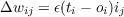
One answer that has occurred to many people over the years is the idea of using the difference between the desired, or target, activation and the obtained activation to drive learning. The idea is to adjust the strengths of the connections so that they will tend to reduce this difference or error measure. Because the rule is driven by differences, we have tended to call it the delta rule. Others have called it the Widrow-Hoff learning rule or the least mean square (LMS) rule (Widrow and Hoff, 1960); it is related to the perceptron convergence procedure of Rosenblatt (1959).

This learning rule, in its simplest form, can be written

(4.4)

where e_i, the error for unit i, is given by

(4.5)

the difference between the teaching input to unit i and its obtained activation.

To see how this rule works, let’s use it to train the five-unit network in Figure 4.1C on the patterns in Figure 4.1D. The training regime is a little different here: For each pattern, we turn the input units on, then we see what effect they have on the output unit; its activation reflects the effects of the current connections in the network. (As before we assume the units are linear.) We compute the difference between the obtained output and the teaching input (Equation 4.5). Then, we adjust the strengths of the connections according to Equation 4.4. We will follow this procedure as we cycle through the four patterns several times, and look at the resulting strengths of the connections as we go. The network is started with initial weights of 0. The results of this process for the first cycle through all four patterns are shown in the first four rows of Figure 4.2.

The first time pattern 0 is presented, the response (that is, the obtained activation of the output unit) is 0, so the error is +1. This means that the changes in the weights are proportional to the activations of the input units. A value of 0.25 was used for the learning rate parameter, so each Δw is ±0.25. These are added to the existing weights (which are 0), so the resulting weights are equal to these initial increments. When pattern 1 is presented, it happens to be uncorrelated with pattern 0, and so again the obtained output is 0. (The output is obtained by summing up the pairwise products of the inputs on the current trial with the weights obtained at the end of the preceding trial.) Again the error is +1, and since all the input units are on in this case, the change in the weight is +0.25 for each input. When these increments are added to the original weights, the result is a value of +0.5 for w₀₄ and w₂₄, and 0 for the other weights. When the next pattern is presented, these weights produce an output of +1. The error is therefore -2, and so relatively larger Δw terms result. Even so, when the final pattern is presented, it produces an output of +1 as well. When the weights are adjusted to take this into account, the weight from input unit 0 is negative and the weight from unit 2 is positive; the other weights are 0. This completes the first sweep through the set of patterns. At this point, the values of the weights are far from perfect; if we froze them at these values, the network would produce 0 output to the first three patterns. It would produce the correct answer (an output of -1) only for the last pattern.

The correct set of weights is approached asymptotically if the training procedure is continued for several more sweeps through the set of patterns. Each of these sweeps, or training epochs, as we will call them henceforth, results in a set of weights that is closer to a perfect solution. To get a measure of the closeness of the approximation to a perfect solution, we can calculate an error measure for each pattern as that pattern is being processed. For each pattern, the error measure is the value of the error (t - a) squared. This measure is then summed over all patterns to get a total sum of squares or tss measure. The resulting error measure, shown for each of the illustrated epochs in Figure 4.2, gets smaller over epochs, as do the changes in the strengths of the connections. The weights that result at the end of 20 epochs of training are very close to the perfect solution values. With more training, the weights converge to these values.

The error-correcting learning rule, then, is much more powerful than the Hebb rule. In fact, it can be proven rather easily that the error-correcting rule will find a set of weights that drives the error as close to 0 as we want for each and every pattern in the training set, provided such a set of weights exists. Many proofs of this theorem have been given; a particularly clear one may be found in Minsky and Papert (1969) (one such proof may be found in PDP:11).

4.1.3 Division of Labor in Error Correcting Learning

It is worth noting an interesting characteristic of error correcting learning rules. This is that, when possible, they divide up the work of driving output units to their correct target values. A simple case of this could arise in the simple network we have already been considering.

Suppose we create a very simple training set consisting of two input patterns and corresponding single desired outputs:

In this case, we see that three of the input units are perfectly correlated with the output and one is uncorrelated with it. If we present these two input patterns repeatedly with a small learning rate, the connection weights will converge to

You can verify that with these connection weights, the network will produce the correct output for both inputs. Now, consider what would happen if the input patterns were:

Here, only one input unit is correlated with the output unit. What will the connection weights converge to in this case? The second, third, and fourth unit cannot help predict the output, so these weights will all be 0. The first unit will have to do all the work, and so the first weight will be 1. While this set of weights would work for the first set of input patterns, the learning rule tends to spread the responsibility or divide the labor among the units that best predict the output. This tendency to ’divide the labor’ among the input units is a characteristic of error correcting learning, and does not occur with the simple Hebbian learning rule because that rule is only sensitive to pairwise input-output correlations.

4.1.4 The Linear Predictability Constraint

We have just noted that the delta rule will find a set of weights that solves a network learning problem, provided such a set of weights exists. What are the conditions under which such a set actually does exist?

Such a set of weights exists only if for each input-pattern-target-pair the target can be predicted from a weighted sum, or linear combination, of the activations of the input units. That is, the set of weights must satisfy

(4.6)

for output unit i in all patterns p.

This constraint (which we called the linear predictability constraint in PDP:17) can be overcome by the use of hidden units, but hidden units cannot be trained using the delta rule as we have described it here because (by definition) there is no teacher for them. Procedures for training such units are discussed in Chapter 5.

Up to this point, we have considered the use of the Hebb rule and the delta rule for training connections coming into a single unit. We now consider how these learning rules produce the characteristics of pattern associator networks.

4.2 THE PATTERN ASSOCIATOR

In a pattern associator, there are two sets of units: input units and output units. There is also a matrix representing the connections from the input units to the output units. A pattern associator is really just an extension of the simple networks we have been considering up to now, in which the number of output units is greater than one and each input unit has a connection to each output unit. An example of an eight-unit by eight-unit pattern associator is shown in Figure 4.3.

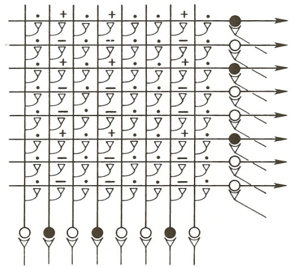
The pattern associator is a device that learns associations between input patterns and output patterns. It is interesting because what it learns about one pattern tends to generalize to other similar patterns. In what follows we will see how this property arises, first in the simplest possible pattern associator: a pattern associator consisting of linear units, trained by the Hebb rule.¹

4.2.1 The Hebb Rule in Pattern Associator Models

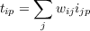
To begin, let us consider the effects of training a network with a single learning trial l, involving an input pattern i_l, and an output pattern o_l. We will use the notational convention that vector names are bolded.

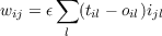
Assuming all the weights in the network are initially 0, we can express the value of each weight as

(4.7)

Note that we are using the variable i_jl to stand for the activation of input unit j in input pattern i_l, and we are using o_il to stand for the activation of output unit i in output pattern o_l. Thus, each weight is just the product of the activation of the input unit times the activation of the output unit in the learning trial l.

In this chapter, many of the formulas are also presented as MATLAB routines to further familiarize the reader with the MATLAB operations. In these routines, the subscript on the vector names will be dropped when clear. Thus, i_l will just be denoted i in the code. Vectors are assumed to be row vectors.

In MATLAB, the above formula (Eq. 4.7) is an outer product:

where the prime is the transpose operator. Dimensions of the outer product are the outer dimensions of the contributing vectors: o′ dims are [8 1], i dims are [1 8], and so W dims are [8 8]. We also adopt the convention that weight matrices are of size [noutputs ninputs].

Now let us present a test input pattern, i_t, and examine the resulting output pattern it produces. Since the units are linear, the activation of output unit i when tested with input pattern i_t is

(4.8)

which is equivalent to

in MATLAB, where o is a column vector. Substituting for w_ij from Equation 4.7 yields

(4.9)

Since we are summing with respect to j in this last equation, we can pull out ϵ and o_il:

(4.10)

Equation 4.10 says that the output at the time of test will be proportional to the output at the time of learning times the sum of the elements of the input pattern at the time of learning, each multiplied by the corresponding element of the input pattern at the time of test.

This sum of products of corresponding elements is called the dot product. It is very important to our analysis because it expresses the similarity of the two patterns i_l and i_t. It is worth noting that we have already encountered an expression similar to this one in Equation 4.2. In that case, though, the quantity was proportional to the correlation of the activations of two units across an ensemble of patterns. Here, it is proportional to the correlation of two patterns across an ensemble of units. It is often convenient to normalize the dot product by taking out the effects of the number of elements in the vectors in question by dividing the dot product by the number of elements. We will call this quantity the normalized dot product. For patterns consisting of all +1s and -1s, it corresponds to the correlation between the two patterns. The normalized dot product has a value of 1 if the patterns are identical, a value of -1 if they are exactly opposite to each other, and a value of 0 if the elements of one vector are completely uncorrelated with the elements of the other. To compute the normalized dot product with MATLAB:

or for two row vectors

We can rewrite Equation 4.10, then, replacing the summed quantity by the normalized dot product of input pattern i_l and input pattern i_t, which we denote by (i_l ⋅i_t)_n:

(4.11)

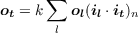
where k = nϵ (n is the number of units). Since Equation 4.11 applies to all of the elements of the output pattern o_t, we can write

(4.12)

In MATLAB, this is

This result is very basic to thinking in terms of patterns since it demonstrates that what is crucial for the performance of the network is the similarity relations among the input patterns–their correlations–rather than their specific properties considered as individuals.² Thus Equation 4.12 says that the output pattern produced by our network at test is a scaled version of the pattern stored on the learning trial. The magnitude of the pattern is proportional to the similarity of the learning and test patterns. In particular, if k = 1 and if the test pattern is identical to the training pattern, then the output at test will be identical to the output at learning.

An interesting special case occurs when the normalized dot product between the learned pattern and the test pattern is 0. In this case, the output is 0: There is no response whatever. Patterns that have this property are called orthogonal or uncorrelated; note that this is not the same as being opposite or anticorrelated.

To develop intuitions about orthogonality, you should compute the normalized dot products of each of the patterns b, c, d, and e below with pattern a:

You will see that patterns b, c, and d are all orthogonal to pattern a; in fact, they are all orthogonal to each other. Pattern e, on the other hand, is not orthogonal to pattern a, but is anticorrelated with it. Interestingly, it forms an orthogonal set with patterns b, c, and d. When all the members of a set of patterns are orthogonal to each other, we call them an orthogonal set.

Now let us consider what happens when an entire ensemble of patterns is presented during learning. In the Hebbian learning situation, the set of weights resulting from an ensemble of patterns is just the sum of the sets of weights resulting from each individual pattern. Note that, in the model we are considering, the output pattern, when provided, is always thought of as clamping the state the output units to the indicated values, so that the existing values of the weights actually play no role in setting the activations of the output units. Given this, after learning trials on a set of input patterns i_l each paired with an output pattern o_l, the value of each weight will be

(4.13)

Thus, the output produced by each test pattern is

(4.14)

In words, the output of the network in response to input pattern t is the sum of the output patterns that occurred during learning, with each pattern’s contribution weighted by the similarity of the corresponding input pattern to the test pattern. Three important facts follow from this:

1. If a test input pattern is orthogonal to all training input patterns, the output of the network will be 0; there will be no response to an input pattern that is completely orthogonal to all of the input patterns that occurred during learning.
2. If a test input pattern is similar to one of the learned input patterns and is uncorrelated with all the others, then the test output will be a scaled version of the output pattern that was paired with the similar input pattern during learning. The magnitude of the output will be proportional to the similarity of the test input pattern to the learned input pattern.
3. For other test input patterns, the output will always be a blend of the training outputs, with the contribution of each output pattern weighted by the similarity of the corresponding input pattern to the test input pattern.

In the exercises, we will see how these properties lead to several desirable features of pattern associator networks, particularly their ability to generalize based on similarity between test patterns and patterns presented during training.

These properties also reflect the limitations of the Hebbian learning rule; when the input patterns used in training the network do not form an orthogonal set, it is not in general possible to avoid contamination, or “cross-talk,” between the response that is appropriate to one pattern and the response that occurs to the others. This accounts for the failure of Hebbian learning with the second set of training patterns considered in Figure 4.1. The reader can check that the input patterns we used in our first training example in Figure 4.1 (which was successful) were orthogonal but that the patterns used in the second example were not orthogonal.

4.2.2 The Delta Rule in Pattern Associator Models

Once again, the delta rule allows us to overcome the orthogonality limitation imposed by the Hebb rule. For the pattern associator case, the delta rule for a particular input-target pair i_l, t_l is

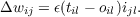(4.15)

which in MATLAB is (again, assuming row vectors)

Therefore the weights that result from an ensemble of learning pairs indexed by l can be written:

(4.16)

It is interesting to compare this to the Hebb rule. Consider first the case where each of the learned patterns is orthogonal to every other one and is presented exactly once during learning. Then o_l will be 0 (a vector of all zeros) for all learned patterns l, and the above formula reduces to

(4.17)

In this case, the delta rule produces the same results as the Hebb rule; the teaching input simply replaces the output pattern from Equation 4.13. As long as the patterns remain orthogonal to each other, there will be no cross-talk between patterns. Learning will proceed independently for each pattern. There is one difference, however. If we continue learning beyond a single epoch, the delta rule will stop learning when the weights are such that they allow the network to produce the target patterns exactly. In the Hebb rule, the weights will grow linearly with each presentation of the set of patterns, getting stronger without bound.

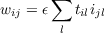
In the case where the input patterns i_l, are not orthogonal, the results of the two learning procedures are more distinct. In this case, though, we can observe the following interesting fact: We can read Equation 4.15 as indicating that the change in the weights that occurs on a learning trial is storing an association of the input pattern with the error pattern; that is, we are adding to each weight an increment that can be thought of as an association between the error for the output unit and the activation of the input unit. To see the implications of this, let’s examine the effects of a learning trial with input pattern i_l paired with output pattern t_l on the output produced by test pattern i_t. The effect of the change in the weights due to this learning trial (as given by Equation 4.15) will be to change the output of some output unit i by an amount proportional to the error that occurred for that unit on the learning trial, e_i, times the dot product of the learned pattern with the test pattern:

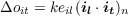
Here k is again equal to ϵ times the number of input units n. In vector notation, the change in the output pattern o_t can be expressed as

Thus, the change in the output pattern at test is proportional to the error vector times the normalized dot product of the input pattern that occurred during learning and the input pattern that occurred during test. Two facts follow from this:

1. If the input on the learning trial is identical to the input on the test trial so that the normalized dot product is 1.0 and if k = 1.0, then the change in the output pattern will be exactly equal to the error pattern. Since the error pattern is equal to the difference between the target and the obtained output on the learning trial, this amounts to one trial learning of the desired association between the input pattern on the training trial and the target on this trial.
2. However, if i_t is different from i_l but not completely different so that (i_l ⋅ i_t)_n n is not equal to either 1 or 0, then the output produced by i_t will be affected by the learning trial. The magnitude of the effect will be proportional to the magnitude of (i_l ⋅i_t)_n.

The second effect–the transfer from learning one pattern to performance on another–may be either beneficial or interfering. Importantly, for patterns of all +1s and -1s, the transfer is always less than the effect on the pattern used on the learning trial itself, since the normalized dot product of two different patterns must be less than the normalized dot product of a pattern with itself. This fact plays a role in several proofs concerning the convergence of the delta rule learning procedure (see Kohonen, 1977, and PDP:11 for further discussion).

4.2.3 Linear Predictability and the Linear Independence Requirement

Earlier we considered the linear predictability constraint for training a single output unit. Since the pattern associator can be viewed as a collection of several different output units, the constraint applies to each unit in the pattern associator. Thus, to master a set of patterns there must exist a set of weights w_ij such that

(4.18)

for all output units i for all target-input pattern pairs p. A consequence of this constraint for the sets of input-output patterns that can be learned by a pattern associator is something we will call the linear independence requirement:

If pattern i_p can be written as a linear combination of the other input patterns, then the output for i_p will be a linear combination of the outputs produced by the other patterns (each other pattern’s contribution to the linear combination will be weighted by it’s similarity to i_p). If this linear combination just happens to be the correct output for i_p, then all is well, but if it is not, the weights will be changed by the delta rule, and this will distort the output pattern produced by one or more of the other patterns in the set.

A pattern that cannot be written as a linear combination of a set of other patterns is said to be linearly independent from these other patterns. When all the members of a set of patterns are linearly independent, we say they form a linearly independent set. To ensure that arbitrary associations to each of a set of input patterns can be learned, the input patterns must form a linearly independent set.

Although this is a serious limitation on what a network can learn, it is worth noting that there are cases in which the response that we need to make to one input pattern can be predictable from the responses that we make to other patterns with which they overlap. In these cases, the fact that the pattern associator produces a response that is a combination of the responses to other patterns can allow it to produce very efficient, often rule-like solutions to the problem of mapping each of a set of input patterns to the appropriate response. We will examine this property of pattern associators in the exercises.

4.2.4 Nonlinear Pattern Associators

Not all pattern associator models that have been studied in the literature make use of the linear activation assumptions we have been using in this analysis. Several different kinds of nonlinear pattern associators (i.e., associators in which the output units have nonlinear activation functions) fall within the general class of pattern associator models. These nonlinearities have effects on performance, but the basic principles that we have observed here are preserved even when these nonlinearities are in place. In particular:

1. Orthogonal inputs are mutually transparent.
2. The learning process converges with the delta rule as long as there is a set of weights that will solve the learning problem.
3. A set of weights that will solve the problem does not always exist.
4. What is learned about one pattern tends to transfer to others.

4.3 THE FAMILY OF PATTERN ASSOCIATOR MODELS

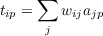
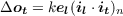
With the above as background, we turn to a brief specification of several members of the class of pattern associator models that are available through the pa program. These are all variants on the pattern associator theme. Each model consists of a set of input units and a set of output units. The activations of the input units are clamped by externally supplied input patterns. The activations of the output units are determined in a single two-phase processing cycle. First, the net input to each output unit is computed. This is the sum of the activations of the input units times the corresponding weights, plus an optional bias term associated with the output unit:

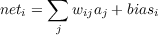(4.19)

4.3.1 Activation Functions

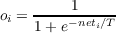
After computing the net input to each output unit, the activation of the output unit is then determined according to an activation function. Several variants are available:

• Linear. Here the activation of output unit i is simply equal to the net input.
• Linear threshold. In this variant, each of the output units is a linear threshold unit; that is, its activation is set to 1 if its net input exceeds 0 and is set to 0 otherwise. Units of this kind were used by Rosenblatt in his work on the perceptron 1959.
• Stochastic. This is the activation function used in PDP:18 and PDP:19. Here, the output is set to 1, with a probability p given by the logistic function:

  (4.20)

  This is the same activation function used in Boltzmann machines.

• Continuous sigmoid. In this variant, each of the output units takes on an activation that is nonlinearly related to its input according to the logistic function:

  (4.21)

  Note that this is a continuous function that transforms net inputs between +∞ and -∞ into real numbers between 0 and 1. This is the activation function used in the back propagation networks we will study in Chapter 5.

4.3.2 Learning Assumptions

Two different learning rules are available in the pa program:

• The Hebb rule. Hebbian learning in the pattern associator model works as follows. Activations of input units are clamped based on an externally supplied input pattern, and activations of the output units are clamped to the values given by some externally supplied target pattern. Learning then occurs by adjusting the strengths of the connections according to the Hebbian rule:

  (4.22)

• The delta rule. Error-correcting learning in the pattern associator model works as follows. Activations of input units are clamped to values determined by an externally supplied input pattern, and activations of the output units are calculated as described earlier. The difference between the obtained activation of the output units and the target activation, as specified in an externally supplied target pattern, is then used in changing the weights according to the following formula:

  (4.23)

4.3.3 The Environment and the Training Epoch

In the pattern associator models, there is a notion of an environment of pattern pairs. Each pair consists of an input pattern and a corresponding output pattern. A training epoch consists of one learning trial on each pattern pair in the environment. On each trial, the input is presented, the corresponding output is computed, and the weights are updated. Patterns may be presented in fixed sequential order or in permuted order within each epoch.

4.3.4 Performance Measures

After processing each pattern, several measures of the output that is produced and its relation to the target are computed. One of these is the normalized dot product of the output pattern with the target. This measure is called the ndp. We have already described this measure quantitatively; here we note that it gives a kind of combined indication of the similarity of two patterns and their magnitudes. In the cases where this measure is most useful-where the target is a pattern of +1s and -1s–the magnitude of the target is fixed and the normalized dot product varies with the similarity of the output to the target and the magnitude of the output itself. To unconfound these factors, we provide two further measures: the normalized vector length, or nvl, of the output vector and the vector correlation, or vcor, of the output vector with the target vector. The nvl measures the magnitude of the output vector, normalizing for the number of elements in the vector. It has a value of 1.0 for vectors consisting of all +1s and -1s. The vcor measures the similarity of the vectors independent of their length; it has a value of 1.0 for vectors that are perfectly correlated, 0.0 for orthogonal vectors, and -1.0 for anticorrelated vectors.

Quantitative definitions of vector length and vector correlation are given in PDP:9 (pp. 376-379). The vector length of vector v, ||v||, is the square root of the dot product of a vector with itself:

and the vector correlation (also called the cosine of the angle between two vectors) is the dot product of the two vectors divided by the product of their lengths:

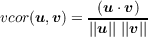
The normalized vector length is obtained by dividing the length by the square root of number of elements. Given these definitions, we can now consider the relationships between the various measures. When the target pattern consists of +1s and -1s, the normalized dot product of the output pattern and the target pattern is equal to the normalized vector length of the output pattern times the vector correlation of the output pattern and the target:

(4.24)

In addition to these measures, we also compute the pattern sum of squares or pss and the total sum of squares or tss. The pss is the sum over all output units of the squared error, where the error for each output unit is the difference between the target and the obtained activation of the unit. This quantity is computed for each pattern processed. The tss is just the sum over the pss values computed for each pattern in the training set. These measures are not very meaningful when learning occurs by the Hebb rule, but they are meaningful when learning occurs by the delta rule.

4.4 IMPLEMENTATION

The pa program implements the pattern associator models in a very straightforward way. The program is initialized by defining a network, as in previous chapters. A PA network consists of a pool of input units (pool(2)) and a pool of output units (pool(3)). pool(1) contains the bias unit which is always on but is not used in these exercises. Connections are allowed from input units to output units only. The network specification file (pa.net) defines the number of input units and output units, as well as the total number of units, and indicates which connections exist. It is also generally necessary to read in a file specifying the set of pattern pairs that make up the environment of the model.

Once the program is initialized, learning occurs through calls to a routine called train. This routine carries out nepochs of training, where the training mode can be selected in the Train options window. strain trains the network with patterns in sequential order, while ptrain permutes the order. The number of epochs can also be set in that window. The routine exits if the total sum of squares measure, tss, is less than some criterion value, ecrit which can also be set in Train options. Here is the train routine:

This calls four other routines: one that sets the input pattern (setinput), one that computes the activations of the output units from the activations of the input units (compute_output), one that computes the error measure (compute_error), and one that computes the various summary statistics (sumstats).

Below we show the compute_output and the compute_error routines. First, compute_output:

The activation function can be selected from the menu in Train options. There are represented in the code as Linear (li), Linear threshold (lt), Stochastic (st), and Continuous Sigmoid (cs). With the linear activation function, the output activation is just the net input. For linear threshold, activation is 1 if the net input is greater than 0, and 0 otherwise. The continuous sigmoid function calls the logistic function shown in Chapter 3. This function returns a number between 0 and 1. For stochastic activation, the logistic activation is first calculated and the result is then used to set the activation of the unit to 0 or 1 using the logistic activation as the probability. The activation function can be specified separately for training and testing via the Train and Test options.

The compute_error function is exceptionally simple for the pa program:

Note that when the targets and the activations of the output units are both specified in terms of 0s and 1s, the error will be 0, 1, or -1.

If learning is enabled (as it is by default in the program, as indicated by the value of the lflag variable which corresponds to the learn checkbox under Train options), the train routine calls the change_weights routine, which actually carries out the learning:

Hebb and Delta are the two possible values of the lrule field under Train options. The lr variable in the code corresponds to the learning rate, which is set by the lrate field in Train options.

Note that for Hebbian learning, we use the target pattern directly in the learning rule, since this is mathematically equivalent to clamping the activations of the output units to equal the target pattern and then using these activations.

4.5 RUNNING THE PROGRAM

The pa program is used much like the other programs we have described in earlier chapters. The main things that are new for this program are the strain and ptrain options for training pattern associator networks.

Training or Testing are selected with the radio button just next to the “options” button. The “Test all” radio button in the upper right corner of the test panel allows you to test the network’s response to all of the patterns in the list of pattern pairs with learning turned off so as not to change the weights while testing.

As in the cs program, the newstart and reset buttons are both available as alternative methods for reinitializing the programs. Recall that reset reinitializes the random number generator with the same seed used the last time the program was initialized, whereas newstart seeds the random number generator with a new random seed. Although there can be some randomness in pa, the problem of local minima does not arise and different random sequences will generally produce qualitatively similar results, so there is little reason to use reset as opposed to newstart.

As mentioned in “Implementation” (Section 4.4), there are several activation functions, and linear is default. Also, Hebb and Delta are alternative rules under lrule in Train options. nepochs in Train options is the number of training epochs run when the “Run” button is pushed in the train panel on the main window. ecrit is the stop criterion value for the error measure. The step-size for the screen updates during training can be set to pattern, cycle or epoch (default) in the train panel on the main window. When pattern is selected and the network is run, the window is updated for every pattern trial of every epoch. If the value is cycle, the screen is updated after processing each pattern and then updated again after the weights are changed for each pattern. Likewise, epoch updates the window just once per epoch after all pattern presentations, which is the fastest but shows the fewest updates.

There are other important options under the Train options. lrate sets the learning rate, which is equivalent to the parameter ϵ from the Background section (4.1). noise determines the amount of random variability added to elements of input and target patterns, and temp is used as the denominator of the logistic function to scale net inputs with the continuous sigmoid and with the stochastic activation function.

There are also several new performance measures displayed on the main window: the normalized dot product, ndp; the normalized vector length measure, nvl; the vector correlation measure, vcor; the pattern sum of squares, pss; and the total sum of squares, tss.

4.5.1 Commands and Parameters

Here follows a more detailed description of the new commands and parameters in pa:

newstart

Button on the Network Viewer, in the train panel. It seeds the random number with a new random seed, and then returns the program to its initial state before any learning occurred. That is, sets all weights to 0, and sets nepochs to 0. Also clears activations and updates the display.

ptrain

Option under trainmode in the Train options. This option, when the network is trained, presents each pattern pair in the pattern list once in each epoch. Order of patterns is rerandomized for each epoch.

reset

Button on the main network window. Same as newstart, but reseeds the random number generator with the same seed that was used last time the network was initialized.

strain

Option under trainmode in the Train options. This option, when the network is trained, pairs are presented in the same, fixed order in each epoch. The order is simply the order in which the pattern pairs are encountered in the list.

Test all

Radio button on the test panel on the Network Viewer. If this option is checked and testing is run, the network will test each testing pattern in sequence. Pressing the step button will present each one by one for better viewing. If it is not checked, the network will test just the selected test pattern. To select a pattern, click on it in the Testing Patterns frame.

ecrit

Parameter in Train options. Error criterion for stopping training. If the tss at the end of an epoch of training is less than this, training stops.

lflag

Check box in Train options. Normally checked, it enables weight updates during learning.

nepochs

Number of training epochs conducted each time the run button is pressed.

Update After

Field in the train and test windows of Network Viewer. Values in the menu are cycle, pattern, and epoch. If the value is cycle, the screen is updated after processing each pattern and then updated again after the weights are changed. This only applies for training. If the value is pattern, the screen is only updated after the weights are changed. If the value is epoch, the screen is updated at the end of each epoch. The number field to the left of this option controls how many cycles, patterns, or epochs occur before an update is made.

actfunction

Field in Train options or Test options. Select from linear, linear threshold, stochastic, or continuous sigmoid.

lrule

Field in Train options. Select between the Hebb and Delta update rules.

lrate

Parameter in Train options. Scales the size of the changes made to the weights. Generally, if there are n input units, the learning rate should be less than or equal to 1∕n.

noise

Parameter in Train and Test options. Range of the random distortion added to each input and target pattern specification value during training and testing. The value added is uniformly distributed in the interval [-noise,+noise].

temp

Denominator used in the logistic function to scale net inputs in both the continuous sigmoid and stochastic modes. Generally, temp can be set to 1. Note that there is only one cycle of processing in pa, so there is no annealing.

4.5.2 State Variables

Sate variables are all associated with the net structure, and some are available for viewing on the Network Viewer. Type “net” at the MATLAB command prompt after starting an exercise to access these variables.

cpname

Name of the current pattern, as given in the pattern file.

epochno

Number of the current epoch; updated at the beginning of each epoch.

error

Vectors of errors, or differences between the current target pattern and the current pattern of activation over the output units.

input

Vector of activations of the input units in the network, based on the current input pattern (subject to the effects of noise). Type net.pool(2).input in the MATLAB command prompt to view this.

ndp

Normalized dot product of the obtained activation vector over the output units and the target vector.

netinput

Vector of net inputs to each output unit. Type net.pool(3).netinput in the MATLAB command prompt to view this.

nvl

Normalized length of the obtained activation vector over the output units.

output

Vector of activations of the output units in the network. Type net.pool(3).output to view.

patno

The number of the current pattern, updated at the beginning of processing the pattern. Note that this is the index of the pattern on the program’s pattern list; when ptrain is used, it is not the same as the pattern’s position within the random training sequence in force for a particular epoch.

pss

Pattern sum of squares, equal to the sum over all output units of the squared difference between the target for each unit and the obtained activation of the unit.

target

Vector of target values for output units, based on the current target pattern, subject to effects of noise.

tss

Total sum of squares, equal to the sum of all patterns so far presented during the current epoch of the pattern sum of squares.

vcor

Vector correlation of the obtained activation vector over the output units and the target vector.

4.6 OVERVIEW OF EXERCISES

In these exercises, we will study several basic properties of pattern associator networks, starting with their tendency to generalize what they have learned to do with one input pattern to other similar patterns; we will explore the role of similarity and the learning of responses to unseen prototypes. These first studies will be done using a completely linear Hebbian pattern associator. Then, we will shift to the linear delta rule associator of the kind studied by Kohonen (1977) and analyzed in PDP:11. We will study what these models can and cannot learn and how they can be used to learn to get the best estimate of the correct output pattern, given noisy input and outputs. Finally, we will examine the acquisition of a rule and an exception to the rule in a nonlinear (stochastic) pattern associator.

Ex4.1. Generalization and Similarity With Hebbian Learning

In this exercise, you will train a linear Hebbian pattern associator on a single input-output pattern pair, and study how its output, after training, is affected by the similarity of the input pattern used at test to the input pattern used during training.

Open MATLAB, and make sure your path is set to include pdptool and all its children, and then move into the pdptool/pa directory. Type “lin” at the MATLAB command prompt. This sets up the network to be a linear Hebbian pattern associator with eight input units and eight output units, starting with initial weights that are all 0. The lin.m file sets the value of the learning rate parameter to 0.125, which is equal to 1 divided by the number of units. With this value, the Hebb rule will learn an association between a single input pattern consisting of all +1s and -1s and any desired output pattern perfectly in one trial.

The file one.pat is loaded and contains a single pattern (or, more exactly, a single input-output pattern pair) to use for training the associator. Both the input pattern and the output pattern are eight-element vectors of +1s and -1s.

Now you can train the network on this first pattern pair for one epoch. Select the train panel, and then select cycle in the train panel. With this option, the program will present the first (and, in this case, only) input pattern, compute the output based on the current weights, and then display the input, output, and target patterns, as well as some summary statistics. If you click “step” in the train panel, the network will pause after the pattern presentation.

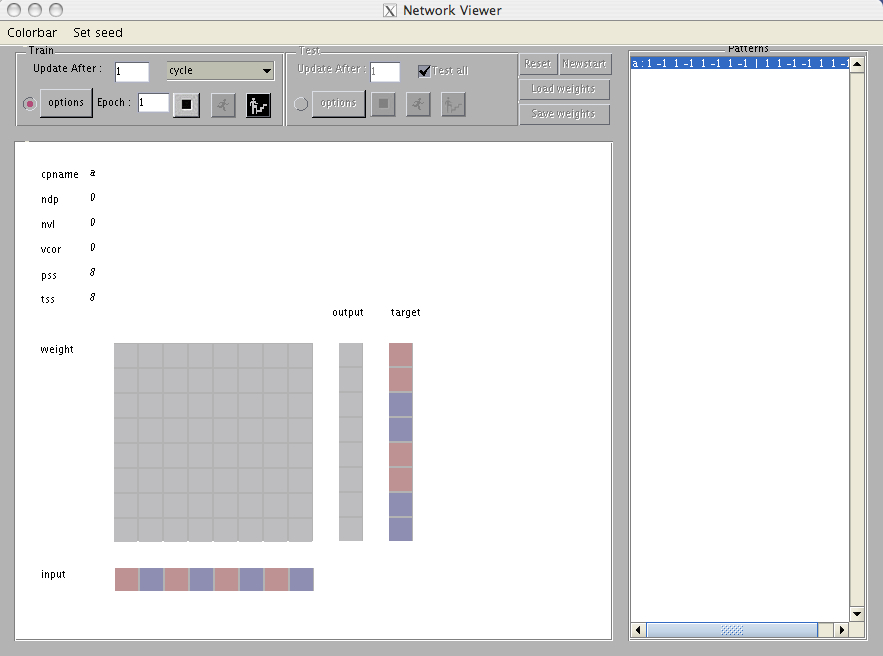
In the upper left corner of the display area, you will see some summary information, including the current ndp, or normalized dot product, of the output obtained by the network with the target pattern; the nvl, or normalized vector length, of the obtained output pattern; and the vcor, or vector correlation, of the output with the target. All of these numbers are 0 because the weights are 0, so the input produces no output at all. Below these numbers are the pss, or pattern sum of squares, and the tss, or total sum of squares. They are the sum of squared differences between the target and the actual output patterns. The first is summed over all output units for the current pattern, and the second is summed over all patterns so far encountered within this epoch (they are, therefore, identical at this point).

Below these entries you will see the weight matrix on the left, with the input vector that was presented for processing below it and the output and target vectors to the right. The display uses shade of red for positive values and shades of blue for negative values as in previous models. A value of +1 or -1 is not very saturated, so that a value can be distinguished over a larger range.

The window of the right of the screen shows the patterns in use for training or test, whichever is selected. Input and target patterns are separated by a vertical separator. You will see that the input pattern shown below the weights matches the single input pattern shown on the right panel and that the target pattern shown to the right of the weights matches the single target pattern to the right of the vertical separator.

If you click step a second time, the target will first be clamped onto the output units, then the weights will be updated according to the Hebbian learning rule:

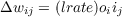(4.25)

Q.4.1.1.

Now, with just this one trial of learning, the network will have “mastered” this particular association, so that if you test it at this point, you will find that, given the learned input, it perfectly reproduces the target. You can test the network using the test command. Simply select the test panel, then click step. In this particular case the display will not change much because in the previous display the output had been clamped to reflect the very target pattern that the network has now computed. The only thing that actually changes in the display are the ndp, vcor, and nvl fields; these will now reflect the normalized dot product and correlation of the computed output with the target and the normalized length of the output. They should all be equal to 1.0 at this point.

You are now ready to test the generalization performance of the network. You can enter patterns into a file. Start by opening the “one.pat” file, copy the existing pattern and paste several times in a new .pat file. Save this file as “gen.pat”. Edit the input pattern entries for the patterns and give each pattern its own name. See Q.4.1.2 for information on the patterns to enter. Leave the target part of the patterns the same. Then, click Test options, click Load new, and load the new patterns for testing.

Q.4.1.2.

If you understand the results you have obtained in this exercise, you understand the basis of similarity-based generalization in one-layer associative networks. In the process, you should come to develop your intuitions about vector similarity and to clearly be able to distinguish uncorrelated patterns from anticorrelated ones.

Ex4.2. Orthogonality, Linear Independence, and Learning

This exercise will expose you to the limitation of a Hebbian learning scheme and show how this limitation can be overcome using the delta rule. For this exercise, you are to set up two different sets of training patterns: one in which all the input patterns form an orthogonal set and the other in which they form a linearly independent, but not orthogonal, set. For both cases, choose the output patterns so that they form an orthogonal set, then arbitrarily assign one of these output patterns to go with each input pattern. In both cases, use only three pattern pairs and make sure that both patterns in each pair are eight elements long. The pattern files you construct in each case should contain three lines formatted like the single line in the one.pat file:

We provide sets of patterns that meet these conditions in the two files ortho.pat and li.pat. However, we want you to make up your own patterns. Save both sets for your use in the exercises in files called myortho.pat and myli.pat. For each set of patterns, display the patterns in a table, then answer each of the next two questions.

Q.4.2.1.

Q.4.2.2.

For the next question, reset your network, and load the pattern set in the file li.pat for both training and testing. Run one epoch of training using the Hebb rule, and save the weights, using a command like:

Then press reset again, and switch to the delta rule. Run one epoch of training at a time, and examine performance at the end of each epoch by testing all patterns.

Q.4.2.3.

Keep running training epochs using the delta rule until the tss measure drops below 0.01. Store the weights in a variable, such as liDeltawts, so that you can display them numerically.

Q.4.2.4.

Hint.

As the final exercise in this set, construct a set of input-output pattern pairs that cannot be learned by a delta rule network, referring to the linear independence requirement and the text in Section 4.2.3 to help you construct an unlearnable set of patterns. Full credit will be given for sets containing more than 2 patterns, such that with all but one of the patterns, the set can be learned, but with all three, the set cannot be learned.

Q.4.2.5.

Hint.

Ex4.3. Learning Central Tendencies

One of the positive features of associator models is their ability to filter out noise in their environments. In this exercise we invite you to explore this aspect of pattern associator networks. For this exercise, you will still be using linear units but with the delta rule and with a relatively small learning rate. You will also be introducing noise into your training patterns.

For this exercise, exit the PDP program and then restart it by typing ct at the command prompt (ct is for “central tendency”). This file sets the learning rate to 0.0125 and uses the Delta rule. It also sets the noise variable to 0.5. This means that each element in each input pattern and in each target pattern will have its activation distorted by a random amount uniformly distributed between +0.5 and -0.5.

Then load in a set of patterns (your orthogonal set from Ex. 4.2 or the patterns in ortho.pat). Then you can see how well the model can do at pulling out the “signals” from the “noise.” The clearest way to see this is by studying the weights themselves and comparing them to the weights acquired with the same patterns without noise added. You can also test with noise turned off; in fact as loaded, noise is turned off for testing, so running a test allows you to see how well the network can do with patterns without noise added.

Q.4.3.1.

Hint.

The results of this simulation are relevant to the theoretical analyses described in PDP:11 and are very similar to those described under “central tendency learning” in PDP:25, where the effects of amnesia (taken as a reduction in connection strength) are considered.

Ex4.4. Lawful Behavior

We now turn to one of the principle characteristics of pattern associator models that has made us take interest in them: their ability to pick up regularities in a set of input-output pattern pairs. The ability of pattern associator models to do this is illustrated in the past-tense learning model, discussed in PDP:18. Here we provide the opportunity to explore this aspect of pattern associator models, using the example discussed in that chapter, namely, the rule of 78 (see PDP:18, pp. 226-234). We briefly review this example here.

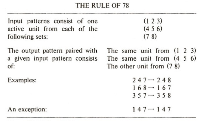
The rule of 78 is a simple rule we invented for the sake of illustration. The rule first defines a set of eight-element input patterns. In each input pattern, one of units 1, 2, and 3 must be on; one of units 4, 5, and 6 must be on; and one of units 7 and 8 must be on. For the sake of consistency with PDP:18, we adopt the convention for this example only of numbering units starting from 1. The rule of 78 also defines a mapping from input to output patterns. For each input pattern, the output pattern that goes with it is the same as the input pattern, except that if unit 7 is on in the input pattern, unit 8 is on in the output and vice versa. Figure 4.5 shows this rule.

The rule of 78 defines 18 input-output pattern pairs. Eighteen arbitrary input-output pattern pairs would exceed the capacity of an eight-by-eight pattern associator, but as we shall see, the patterns that exemplify the rule of 78 can easily be learned by the network.

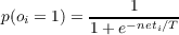
The version of the pattern associator used for this example follows the assumptions we adopted in PDP:18 for the past-tense learning model. Input units are binary and are set to 1 or 0 according to the input pattern. The output units are binary, stochastic units and take on activation values of 0 or 1 with probability given by the logistic function:

(4.26)

where T is equivalent to the Temp parameter in Train and Test options. Note that, although this function is the same as for the Boltzmann machine, the calculation of the output is only done once, as in other versions of the pattern associator; there is no annealing, so Temp is just a scaling factor.

Learning occurs according to the delta rule, which in this case is equivalent to the perceptron convergence procedure because the units are binary. Thus, when an output unit should be on (target is 1) but is not (activation is 0), an increment of size lrate is added to the weight coming into that unit from each input unit that is on. When an output unit should be off (target is 0) but is not (activation is 1), an increment of size lrate is subtracted from the weight coming into that unit from each input unit that is on.

For this example, we follow PDP:18 and use Temp of 1 and a learning rate of .05. (The simulations that you will do here will not conform to the example in PDP:18 in all details, since in that example an approximation to the logistic function was used. The basic features of the results are the same, however.)

To run this example, exit the PDP system if running, and then enter

at the command prompt. This will read in the appropriate network specification file (in 8X8.net) and the 18 patterns that exemplify the rule of 78, then display these on the screen to the right of the weight matrix. Since the units are binary, there is only a single digit of precision for both the input, output, and target units.

You should now be ready to run the exercise. The variable Epochs is initialized to 10, so if you press the Run button, 10 epochs of training will be run. We recommend using ptrain because it does not result in a consistent bias in the weights favoring the patterns later in the pattern list. If you want to see the screen updated once per pattern, set the Update After field in the train panel to be “pattern” instead of “epoch.” If “pattern” is selected, the screen is updated once per pattern after the weights have been adjusted, so you should see the weights and the input, output, and target bits changing. The pss and tss (which in this case indicate the number of incorrect output bits) will also be displayed once per pattern.

Q.4.4.1.

At this point you should be able to see the solution to the rule of 78 patterns emerging. Generally, there are large positive weights between input units and corresponding output units, with unit 7 exciting unit 8 and unit 8 exciting unit 7. You’ll also see rather large inhibitory weights from each input unit to each other unit within the same subgroup (i.e., 1, 2, and 3; 4, 5, and 6; and 7 and 8). Run another 40 or so epochs, and a subtler pattern will begin to emerge.

Q.4.4.2.

At this point, you have watched a simple PDP network learn to behave in accordance with a simple rule, using a simple, local learning scheme; that is, it adjusts the strength of each connection in response to its errors on each particular learning experience, and the result is a system that exhibits lawful behavior in the sense that it conforms to the rule.

For the next part of the exercise, you can explore the way in which this kind of pattern associator model captures the three-stage learning phenomenon exhibited by young children learning the past tense in the course of learning English as their first language. To briefly summarize this phenomenon: Early on, children know only a few words in the past tense. Many of these words happen to be exceptions, but at this point children tend to get these words correct. Later in development, children begin to use a much larger number of words in the past tense, and these are predominantly regular. At this stage, they tend to overregularize exceptions. Gradually, over the course of many years, these exceptions become less frequent, but adults have been known to say things like ringed or taked, and lower-frequency exceptions tend to lose their exceptionality (i.e., to become regularized) over time.

The 78 model can capture this pattern of results; it is interesting to see it do this and understand how and why this happens. For this part of the exercise, you will want to reset the weights, and read in the file hf.pat, which contains a exception pattern (147-→147) and one regular pattern (258-→257). If we imagine that the early experience of the child consists mostly of exposure to high-frequency words, a large fraction of which are irregular (8 of the 10 most frequent verbs are irregular), this approximates the early experience the child might have with regular and irregular past-tense forms. If you run 30 epochs of training using ptrain with these two patterns, you will see a set of weights that allows the model to often set each output bit correctly, but not reliably. At this point, you can read in the file all.pat, which contains these two pattern pairs, plus all of the other pairs that are consistent with the rule of 78. This file differs from the 78.pat file only in that the input pattern 147 is associated with the “exceptional” output pattern 147 instead of what would be the “regular” corresponding pattern 148. Save the weights that resulted from learning hf.pat. Then read in all.pat and run 10 more epochs.

Q.4.4.3.

One way to think about what has happened in learning the all.pat stimuli is that the 17 regular patterns are driving the weights in one direction and the single exception pattern is fighting a lonely battle to try to drive the weights in a different direction, at least with respect to the activation of units 7 and 8. Since eight of the input patterns have unit 7 on and “want” output unit 8 to be on and unit 7 to be off and only one input pattern has input unit 7 on and wants output unit 7 on and output unit 8 off, it is hardly a fair fight.

If you run more epochs (upwards of 300), though, you will find that the network eventually finds a compromise solution that satisfies all of the patterns.

Q.4.4.4.

Ex4.5. Learning quasi-regular exceptions

Pinker and Ullman (2002) argue for a two-system model, in which a connectionist like system deals with exceptions, but there is a separate “procedural” system for rules. Consider the response to this position contained in the short reply to Pinker and Ullman (2002) by McClelland and Patterson (2002).

Q.4.5.1.

4.6.1 Further Suggestions for Exercises

There are other exercises for further exploration. In the 78 exercise just described, there was only one exception pattern, and when vocabulary size increased, the ratio of regular to exception patterns increased from 1:1 to 17:1. Pinker and Prince (1988) have shown that, in fact, as vocabulary size increases, the ratio of regular to exception verbs stays roughly constant at 1:1. One interesting exercise is to set up an analog of this situation. Start training the network with one regular and one exception pattern, then increase the “vocabulary” by introducing new regular patterns and new exceptions. Note that each exception should be idiosyncratic; if all the exceptions were consistent with each other, they would simply exemplify a different rule. You might try an exercise of this form, setting up your own correspondence rules, your own exceptions, and your own regime for training.

You can also explore other variants of the pattern associator with other kinds of learning problems. One thing you can do easily is see whether the model can learn to associate each of the individuals from the Jets and Sharks example in Chapter 2 with the appropriate gang (relying only on their properties, not their names; the files jets.tem, jets.net, and jets.pat are available for this purpose). Also, you can play with the continuous sigmoid (or logistic) activation function.