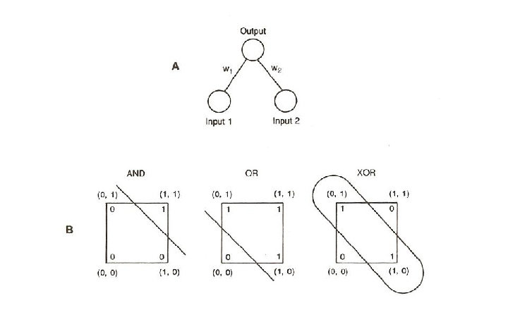
Figure 5.1: The one-layer perceptron analyzed by Minsky and Papert. (From
Perceptrons by M. L Minsky and S. Papert, 1969, Cambridge, MA: MIT Press.
Copyright 1969 by MIT Press. Reprinted by permission.)
In this chapter, we introduce the back propagation learning procedure for learning internal representations. We begin by describing the history of the ideas and problems that make clear the need for back propagation. We then describe the procedure, focusing on the goal of helping the student gain a clear understanding of gradient descent learning and how it is used in training PDP networks. The exercises are constructed to allow the reader to explore the basic features of the back propagation paradigm. At the end of the chapter, there is a separate section on extensions of the basic paradigm, including three variants we call cascaded back propagation networks, recurrent networks, and sequential networks. Exercises are provided for each type of extension.
The pattern associator described in the previous chapter has been known since the late 1950s, when variants of what we have called the delta rule were first proposed. In one version, in which output units were linear threshold units, it was known as the perceptron (cf. Rosenblatt, 1959, 1962). In another version, in which the output units were purely linear, it was known as the LMS or least mean square associator (cf. Widrow and Hoff, 1960). Important theorems were proved about both of these versions. In the case of the perceptron, there was the so-called perceptron convergence theorem. In this theorem, the major paradigm is pattern classification. There is a set of binary input vectors, each of which can be said to belong to one of two classes. The system is to learn a set of connection strengths and a threshold value so that it can correctly classify each of the input vectors. The basic structure of the perceptron is illustrated in Figure 5.1. The perceptron learning procedure is the following: An input vector is presented to the system (i.e., the input units are given an activation of 1 if the corresponding value of the input vector is 1 and are given 0 otherwise). The net input to the output unit is computed: net = ∑ iwiii. If net is greater than the threshold θ, the unit is turned on, otherwise it is turned off. Then the response is compared with the actual category of the input vector. If the vector was correctly categorized, then no change is made to the weights. If, however, the output turns on when the input vector is in category 0, then the weights and thresholds are modified as follows: The threshold is incremented by 1 (to make it less likely that the output unit will come on if the same vector were presented again). If input ii is 0, no change is made in the weight Wi (that weight could not have contributed to its having turned on). However, if ii = 1, then Wi is decremented by 1. In this way, the output will not be as likely to turn on the next time this input vector is presented. On the other hand, if the output unit does not come on when it is supposed to, the opposite changes are made. That is, the threshold is decremented, and those weights connecting the output units to input units that are on are incremented.
Mathematically, this amounts to the following: The output, o, is given by
| o = 1 | if net < θ | ||
| o = 0 | otherwise |
where p indexes the particular pattern being tested, tp is the target value indicating the correct classification of that input pattern, and δp is the difference between the target and the actual output of the network. Finally, the changes in the weights, Δwi. are given by

The remarkable thing about this procedure is that, in spite of its simplicity, such a system is guaranteed to find a set of weights that correctly classifies the input vectors if such a set of weights exists. Moreover, since the learning procedure can be applied independently to each of a set of output units, the perceptron learning procedure will find the appropriate mapping from a set of input vectors onto a set of output vectors if such a mapping exists. Unfortunately, as indicated in Chapter 4, such a mapping does not always exist, and this is the major problem for the perceptron learning procedure.
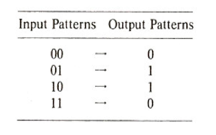
In their famous book Perceptrons, Minsky and Papert (1969) document the limitations of the perceptron. The simplest example of a function that cannot be computed by the perceptron is the exclusive-or (XOR), illustrated in Figure 5.2. It should be clear enough why this problem is impossible. In order for a perceptron to solve this problem, the following four inequalities must be satisfied:
| 0 × w1 + 0 × w2 | < θ → 0 < θ | ||
| 0 × w1 + 1 × w2 | > θ → w1 > θ | ||
| 1 × w1 + 0 × w2 | > θ → w2 > θ | ||
| 1 × w1 + 1 × w2 | < θ → w1 + w2 < θ | ||
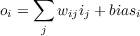
Obviously, we can’t have both w1 and w2 greater than θ while their sum, w1 + w2, is less than θ. There is a simple geometric interpretation of the class of problems that can be solved by a perceptron: It is the class of linearly separable functions. This can easily be illustrated for two dimensional problems such as XOR. Figure 5.3 shows a simple network with two inputs and a single output and illustrates three two-dimensional functions: the AND, the OR, and the XOR. The first two can be computed by the network; the third cannot. In these geometrical representations, the input patterns are represented as coordinates in space. In the case of a binary two-dimensional problem like XOR, these coordinates constitute the vertices of a square. The pattern 00 is represented at the lower left of the square, the pattern 10 as the lower right, and so on. The function to be computed is then represented by labeling each vertex with a 1 or 0 depending on which class the corresponding input pattern belongs to. The perceptron can solve any function in which a single line can be drawn through the space such that all of those labeled ”0” are on one side of the line and those labeled ”1” are on the other side. This can easily be done for AND and OR, but not for XOR. The line corresponds to the equation i1w1 + i2w2 = θ. In three dimensions there is a plane, i1w1 + i2w2 + i3w3 = θ, that corresponds to the line. In higher dimensions there is a corresponding hyperplane, ∑ iwiii = θ. All functions for which there exists such a plane are called linearly separable.
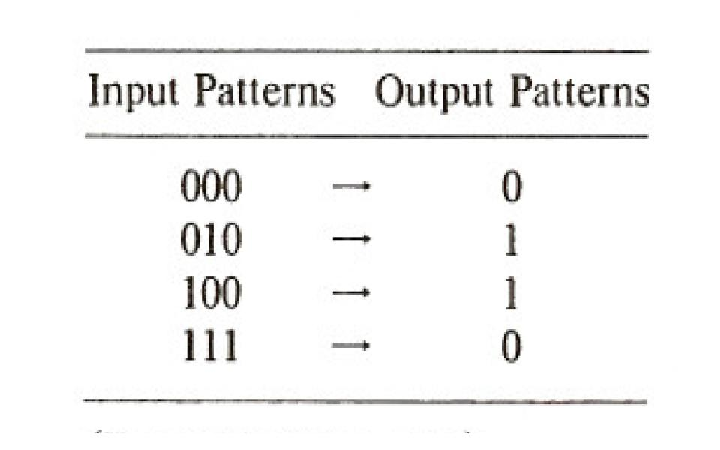
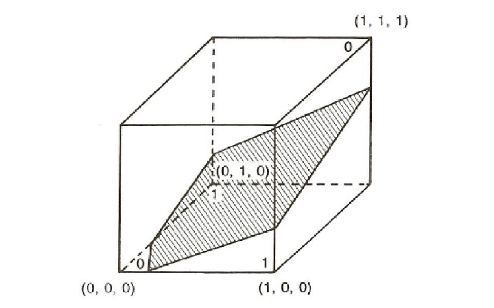
Now consider the function in Figure 5.4 and shown graphically in Figure 5.5. This is a three-dimensional problem in which the first two dimensions are identical to the XOR and the third dimension is the AND of the first two dimensions. (That is, the third dimension is 1 whenever both of the first two dimensions are 1, otherwise it is 0). Figure 5.5 shows how this problem can be represented in three dimensions. The figure also shows how the addition of the third dimension allows a plane to separate the patterns classified in category 0 from those in category 1. Thus, we see that the XOR is not solvable in two dimensions, but if we add the appropriate third dimension, that is, the appropriate new feature, the problem is solvable. Moreover, as indicated in Figure 5.6, if you allow a multilayered perceptron, it is possible to take the original two-dimensional problem and convert it into the appropriate three-dimensional problem so it can be solved. Indeed, as Minsky and Papert knew, it is always possible to convert any unsolvable problem into a solvable one in a multilayer perceptron. In the more general case of multilayer networks, we categorize units into three classes: input units, which receive the input patterns directly; output units, which have associated teaching or target inputs; and hidden units, which neither receive inputs directly nor are given direct feedback. This is the stock of units from which new features and new internal representations can be created. The problem is to know which new features are required to solve the problem at hand. In short, we must be able to learn intermediate layers. The question is, how? The original perceptron learning procedure does not apply to more than one layer. Minsky and Papert believed that no such general procedure could be found. To examine how such a procedure can be developed it is useful to consider the other major one-layer learning system of the 1950s and early 1960s, namely, the least-mean-square (LMS) learning procedure of Widrow and Hoff (1960).

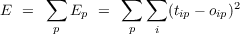
The LMS procedure makes use of the delta rule for adjusting connection weights; the perceptron convergence procedure is very similar, differing only in that linear threshold units are used instead of units with continuous-valued outputs. We use the term LMS procedure here to stress the fact that this family of learning rules may be viewed as minimizing a measure of the error in their performance. The LMS procedure cannot be directly applied when the output units are linear threshold units (like the perceptron). It has been applied most often with purely linear output units. In this case the activation of an output unit, oi, is simply given by
Note the introduction of the bias term which serves the same function as the threshold θ in the Perceptron. Providing a bias equal to -θ and setting the threshold to 0 is equivalent to having a threshold of θ. The bias is also equivalent to a weight to the output unit from an input unit that is always on.
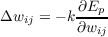
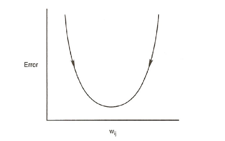
The error measure being minimised by the LMS procedure is the summed squared error. That is, the total error, E, is defined to be
where the index p ranges over the set of input patterns, i ranges over the set of output units, and Ep represents the error on pattern p. The variable tip is the desired output, or target, for the ith output unit when the pth pattern has been presented, and oip is the actual output of the ith output unit when pattern p has been presented. The object is to find a set of weights that minimizes this function. It is useful to consider how the error varies as a function of any given weight in the system. Figure 5.7 illustrates the nature of this dependence. In the case of the simple single-layered linear system, we always get a smooth error function such as the one shown in the figure. The LMS procedure finds the values of all of the weights that minimize this function using a method called gradient descent. That is, after each pattern has been presented, the error on that pattern is computed and each weight is moved ”down” the error gradient toward its minimum value for that pattern. Since we cannot map out the entire error function on each pattern presentation, we must find a simple procedure for determining, for each weight, how much to increase or decrease each weight. The idea of gradient descent is to make a change in the weight proportional to the negative of the derivative of the error, as measured on the current pattern, with respect to each weight.1 Thus the learning rule becomes
where k is the constant of proportionality. Interestingly, carrying out the derivative of the error measure in Equation 1 we get

where ϵ = 2k and δip = (tip - oip) is the difference between the target for unit i on pattern p and the actual output produced by the network. This is exactly the delta learning rule described in Equation 15 from Chapter 4. It should also be noted that this rule is essentially the same as that for the perceptron. In the perceptron the learning rate was 1 (i.e., we made unit changes in the weights) and the units were binary, but the rule itself is the same: the weights are changed proportionally to the difference between target and output times the input. If we change each weight according to this rule, each weight is moved toward its own minimum and we think of the system as moving downhill in weight-space until it reaches its minimum error value. When all of the weights have reached their minimum points, the system has reached equilibrium. If the system is able to solve the problem entirely, the system will reach zero error and the weights will no longer be modified. If the network is unable to get the problem exactly right, it will find a set of weights that produces as small an error as possible.
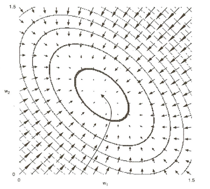
In order to get a fuller understanding of this process it is useful to carefully consider the entire error space rather than a one-dimensional slice. In general this is very difficult to do because of the difficulty of depicting and visualizing high-dimensional spaces. However, we can usefully go from one to two dimensions by considering a network with exactly two weights. Consider, as an example, a linear network with two input units and one output unit with the task of finding a set of weights that comes as close as possible to performing the function OR. Assume the network has just two weights and no bias terms like the network in Figure 5.3A. We can then give some idea of the shape of the space by making a contour map of the error surface. Figure 5.8 shows the contour map. In this case the space is shaped like a kind of oblong bowl. It is relatively flat on the bottom and rises sharply on the sides. Each equal error contour is elliptically shaped. The arrows around the ellipses represent the derivatives of the two weights at those points and thus represent the directions and magnitudes of weight changes at each point on the error surface. The changes are relatively large where the sides of the bowl are relatively steep and become smaller and smaller as we move into the central minimum. The long, curved arrow represents a typical trajectory in weight-space from a starting point far from the minimum down to the actual minimum in the space. The weights trace a curved trajectory following the arrows and crossing the contour lines at right angles.
The figure illustrates an important aspect of gradient descent learning. This is the fact that gradient descent involves making larger changes to parameters that will have the biggest effect on the measure being minimized. In this case, the LMS procedure makes changes to the weights proportional to the effect they will have on the summed squared error. The resulting total change to the weights is a vector that points in the direction in which the error drops most steeply.
Although this simple linear pattern associator is a useful model for understanding the dynamics of gradient descent learning, it is not useful for solving problems such as the XOR problem mentioned above. As pointed out in PDP:2, linear systems cannot compute more in multiple layers than they can in a single layer. The basic idea of the back propagation method of learning is to combine a nonlinear perceptron-like system capable of making decisions with the objective error function of LMS and gradient descent. To do this, we must be able to readily compute the derivative of the error function with respect to any weight in the network and then change that weight according to the rule
How can this derivative be computed? First, it is necessary to use a differentiable
output function, rather than the threshold function used in the perceptron
convergence procedure. A common choice, and one that allows us to relate
back-propagation learning to probabilistic inference, is to use the logistic function
f(neti) =  . Given a choice of f, we can then determine the partial
derivative of the Error with respect to a weight coming to an output unit i from a
unit j that projects to it.
. Given a choice of f, we can then determine the partial
derivative of the Error with respect to a weight coming to an output unit i from a
unit j that projects to it.
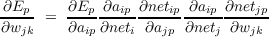
We can use the chain rule to compute the partial derivative of the error with respect to our particular weight wij:
Now, Ep = ∑
i(tip - aip)2, so that  is equal to -2(tip - aip).
ai = f(neti),2
and, so that we can leave f unspecified for the moment, we write f′(neti) to
represent its derivative evaluated at neti. Finally, neti = ∑
jajwij, and its partial
derivative of the net input with respect to wij is just aj. In sum, then we
have
is equal to -2(tip - aip).
ai = f(neti),2
and, so that we can leave f unspecified for the moment, we write f′(neti) to
represent its derivative evaluated at neti. Finally, neti = ∑
jajwij, and its partial
derivative of the net input with respect to wij is just aj. In sum, then we
have
Let us use δip to represent (tip - aip)f′(netip). δip is proportional to (minus)
the partial derivative of the error with respect to the net input to unit i in
pattern p,  . Substituting this into the above expression, we can now
write:
. Substituting this into the above expression, we can now
write:
This generalizes the delta rule from the LMS procedure to the case where there is a non-linearity applied to the output units, with the δ terms now defined so as to take this non-linearity into account.
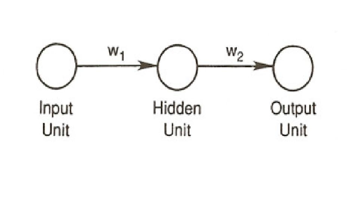
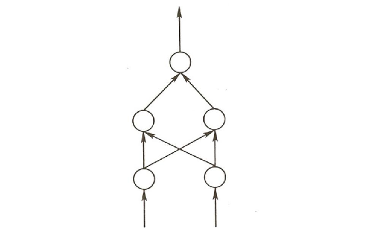
Now let us consider a weight that projects from an input unit k to a hidden unit j, which in turn projects to an output unit, i in a very simple network consisting of only one unit at each of these three layers (see Figure 5.9). We can ask, what is the partial derivative of the error on the output unit i with respect to a change in the weight wjk to the hidden unit from the input unit? It may be helpful to talk yourself informally through the series of effects changing such a weight would have on the error in this case. It should be obvious that if you increase the weight to the hidden unit from the input unit, that will increase the net input to the hidden unit j by an amount that depends on the activation of the input unit k. If the input unit were inactive, the change in the weight would have no effect; the stronger the activation of the input unit, the stronger the effect of changing the weight on the net input to the hidden unit. This change, you should also see, will in turn increase the activation of the hidden unit; the amoung of the increase will depend on the slope (derivative) of the unit’s activation function evaluated at the current value of its net input. This change in the activation with then affect the net input to the output unit i by an amount depending on the current value of the weight to unit i from unit j. This change in the net input to unit i will then affect the activation of unit i by an amount proportional to the derivative of its activation function evaluated at the current value of its net input. This change in the activation of the output unit will then affect the error by an amount proportional to the difference between the target and the current activation of the output unit.
The above is an intuitive account of corresponding to the series of factors you get when you apply the chain rule to unpack the partial derivative of the error at the output unit with respect to a change in the weight to the hidden unit from the input unit. Applying this to the case of the error on pattern p, we would write
The factors in the chain are given in the reverse order from the verbal description above since this is how they will actually be calculated using back propagation. The first two factors on the right correspond to the last two links of the chain described above, and are equal to the δ term for output unit i as previously discussed. The third factor is equal to the weight to output unit i from hidden unit j; and the fourth factor corresponds to the derivative of the activation function of the hidden unit, evaluated at its net input given the current pattern p, f′(netjp). Taking these four factors together they correspond to (minus) the partial derivative of the error at output unit i with respect to the net input to hidden unit j.
Now, if there is more than one output unit, the partial derivative of the error across all of the output units is just equal to the sum of the partial derivatives of the error with respect to each of the output units:
The equation above is the core of the back propagation process and we call it the BP Equation for future reference.
Because  equals akp, the partial derivative of the error with respect to the
weight then becomes:
equals akp, the partial derivative of the error with respect to the
weight then becomes:
Although we have not demonstrated it here, it is easy to show that, with more layers, the correct δ term for each unit j in a given layer of a feed-forward network is always equal to the derivative of the activation function of the unit evaluated at the current value of its net input, times the sum over the forward connections from that unit of the product of the weight on each forward connection times the delta term at the receiving end of that connection; i.e., the δ terms for all layers are determined by applying the BP Equation.
Thus, once delta terms have been computed at the output layers of a feedforward network, the BP equation can be used iteratively to calculate δ terms backward across many layers of weights, and to specify how each weight should be changed to perform gradient decent. Thus we now have a generalized version of the delta rule that specifies a procedure for changing all the weights in all laters of a feed forward network: If we adjust the weight to each output unit i from each unit j projecting to it, by an amount proportional to δipajp, where δj is defined recursively as discussed above, we will be performing gradient descent in E: We will be adjusting each weight in proportion to (minus) the effect that its adjustment would have on the error.
The application of the back propagation rule, then, involves two phases: During the first phase the input is presented and propagated forward through the network to compute the output value aip for each unit. This output is then compared with the target, and scaled by the derivative of the activation function, resulting in a δ term for each output unit. The second phase involves a backward pass through the network (analogous to the initial forward pass) during which the δ term is computed for each unit in the network. This second, backward pass allows the recursive computation of δ as indicated above. Once these two phases are complete, we can compute, for each weight, the product of the δ term associated with the unit it projects to times the activation of the unit it projects from. Henceforth we will call this product the weight error derivative since it is proportional to (minus) the derivative of the error with respect to the weight. As will be discussed later, these weight error derivatives can then be used to compute actual weight changes on a pattern-by-pattern basis, or they may be accumulated over the ensemble of patterns with the accumulated sum of its weight error derivatives then being applied to each of the weights.
Adjusting bias weights. Of course, the generalized delta rule can also be used to learn biases, which we treat as weights from a special “bias unit” that is always on. A bias weight can project from this unit to any unit in the network, and can be adjusted like any other weight, with the further stipulation that the activation of the sending unit in this case is always fixed at 1.
The activation function. As stated above, the derivation of the back propagation learning rule requires that the derivative of the activation function, f′(neti) exists. It is interesting to note that the linear threshold function, on which the perceptron is based, is discontinuous and hence will not suffice for back propagation. Similarly, since a network with linear units achieves no advantage from hidden units, a linear activation function will not suffice either. Thus, we need a continuous, nonlinear activation function. In most of our work on back propagation and in the program presented in this chapter, we have used the logistic activation function.
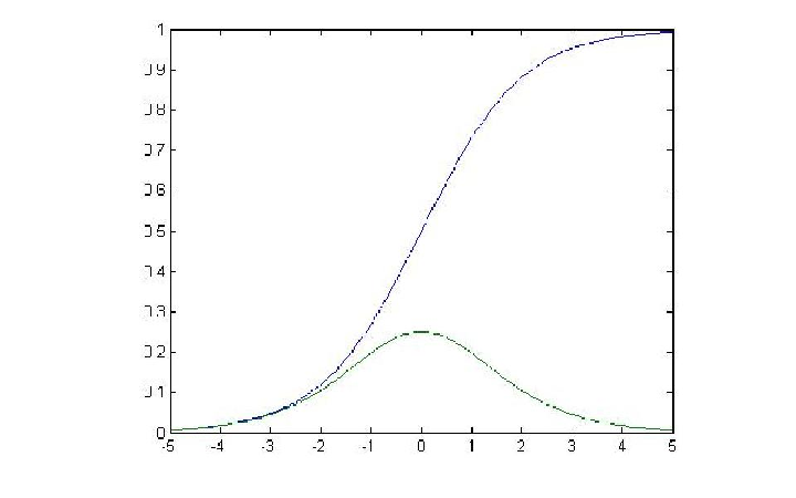
In order to apply our learning rule, we need to know the derivative of this function with respect to its net input. It is easy to show that this derivative is equal to aip(1 - aip). This expression can simply be substituted for f′(net) in the derivations above.
It should be noted that aip(1 -aip) reaches its maximum when aip = 0.5 and goes to 0 as aip approaches 0 or 1 (see Figure 5.10). Since the amount of change in a given weight is proportional to this derivative, weights will be changed most for those units that are near their midrange and, in some sense, not yet committed to being either on or off. This feature can sometimes lead to problems for backpropagation learning, and the problem can be especially serious at the output layer. If the weights in a network at some point during learning are such that a unit that should be on is completely off (or a unit that should be off is completely on) the error at that unit is large but paradoxically the delta term at that unit is very small, and so no error signal is propagated back through the network to correct the problem.
An improved error measure. There are various ways around the problem just noted above. One is to simply leave the f′(neti) term out of the calculation of delta terms at the output units. In practice, this solves the problem, but it seems like a bit of a hack.
Interestingly, however, if the error measure E is replaced by a different measure, called the ’cross-entropy’ error, here called CE, we obtain an elegant result. The cross-entropy error for pattern p is defined as
![CE = - ∑ [t log(a )+ (1- t )log(1- a )]
p i ip ip ip ip](handbook85x.png)
If the target value tip is thought of as a binary random variable having value one with probability pip, and the activation of the output unit aip is construed as representing the network’s estimate of that probability, the cross-entropy measure corresponds to the negative logarithm of the probability of the observed target values, given the current estimates of the pip’s. Minimizing the cross-entropy error corresponds to maximizing the probability of the observed target values. The maximum is reached when for all i and p, aip = pip.
Now very neatly, it turns out that the derivative of CEp with respect to aip is
![[ ]
tip- (1--tip)-
- aip - (1- aip) .](handbook86x.png)
When this is multiplied times the derivative of the logistic function evaluated at the net input, aip(1 -aip), to obtain the corresponding δ term δip, several things cancel out and we are left with

This is the same expression for the δ term we would get using the standard sum squared error measure E, if we simply ignored the derivative of the activation function! Because using cross entropy error seems more appropriate than summed squared error in many cases and also because it often works better, we provide the option of using the cross entropy error in the pdptool back propagation simulator.
Even using cross-entropy instead of sum squared error, it sometimes happens that hidden units have strong learned input weights that ’pin’ their activation against 1 or 0, and in that case it becomes effectively impossible to propagate error back through these units. Different solutions to this problem have been proposed. One is to use a small amount of weight decay to prevent weights from growing too large. Another is to add a small constant to the derivative of the activation function of the hidden unit. This latter method works well, but is often considered a hack, and so is not implemented in the pdptool software. Weight decay is available in the software, however, and is described below.
Local minima. Like the simpler LMS learning paradigm, back propagation is a gradient descent procedure. Essentially, the system will follow the contour of the error surface, always moving downhill in the direction of steepest descent. This is no particular problem for the single-layer linear model. These systems always have bowl-shaped error surfaces. However, in multilayer networks there is the possibility of rather more complex surfaces with many minima. Some of the minima constitute complete solutions to the error minimization problem, in the sense at these minima the system has reached a completely errorless state. All such minima are global minima. However, it is possible for there to be some residual errror at the bottom of some of the minima. In this case, a gradient descent method may not find the best possible solution to the problem at hand.
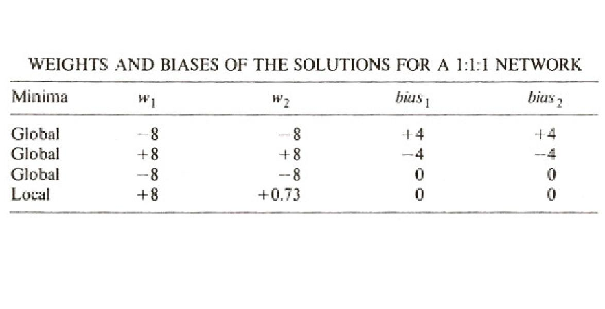
Part of the study of back propagation networks and learning involves a study of how frequently and under what conditions local minima occur. In networks with many hidden units, local minima seem quite rare. However with few hidden units, local minima can occur. The simple 1:1:1 network shown in Figure 5.9 can be used to demonstate this phenomenon. The problem posed to this network is to copy the value of the input unit to the output unit. There are two basic ways in which the network can solve the problem. It can have positive biases on the hidden unit and on the output unit and large negative connections from the input unit to the hidden unit and from the hidden unit to the output unit, or it can have large negative biases on the two units and large positive weights from the input unit to the hidden unit and from the hidden unit to the output unit. These solutions are illustrated in Figure 5.11. In the first case, the solution works as follows: Imagine first that the input unit takes on a value of 0. In this case, there will be no activation from the input unit to the hidden unit, but the bias on the hidden unit will turn it on. Then the hidden unit has a strong negative connection to the output unit so it will be turned off, as required in this case. Now suppose that the input unit is set to 1. In this case, the strong inhibitory connection from the input to the hidden unit will turn the hidden unit off. Thus, no activation will flow from the hidden unit to the output unit. In this case, the positive bias on the output unit will turn it on and the problem will be solved. Now consider the second class of solutions. For this case, the connections among units are positive and the biases are negative. When the input unit is off, it cannot turn on the hidden unit. Since the hidden unit has a negative bias, it too will be off. The output unit, then, will not receive any input from the hidden unit and since its bias is negative, it too will turn off as required for zero input. Finally, if the input unit is turned on, the strong positive connection from the input unit to the hidden unit will turn on the hidden unit. This in turn will turn on the output unit as required. Thus we have, it appears, two symmetric solutions to the problem. Depending on the random starting state, the system will end up in one or the other of these global minima.
Interestingly, it is a simple matter to convert this problem to one with one local and one global minimum simply by setting the biases to 0 and not allowing them to change. In this case, the minima correspond to roughly the same two solutions as before. In one case, which is the global minimum as it turns out, both connections are large and negative. These minima are also illustrated in Figure 5.11. Consider first what happens with both weights negative. When the input unit is turned off, the hidden unit receives no input. Since the bias is 0, the hidden unit has a net input of 0. A net input of 0 causes the hidden unit to take on a value of 0.5. The 0.5 input from the hidden unit, coupled with a large negative connection from the hidden unit to the output unit, is sufficient to turn off the output unit as required. On the other hand, when the input unit is turned on, it turns off the hidden unit. When the hidden unit is off, the output unit receives a net input of 0 and takes on a value of 0.5 rather than the desired value of 1.0. Thus there is an error of 0.5 and a squared error of 0.25. This, it turns out, is the best the system can do with zero biases. Now consider what happens if both connections are positive. When the input unit is off, the hidden unit takes on a value of 0.5. Since the output is intended to be 0 in this case, there is pressure for the weight from the hidden unit to the output unit to be small. On the other hand, when the input unit is on, it turns on the hidden unit. Since the output unit is to be on in this case, there is pressure for the weight to be large so it can turn on the output unit. In fact, these two pressures balance off and the system finds a compromise value of about 0.73. This compromise yields a summed squared error of about 0.45—a local minimum.
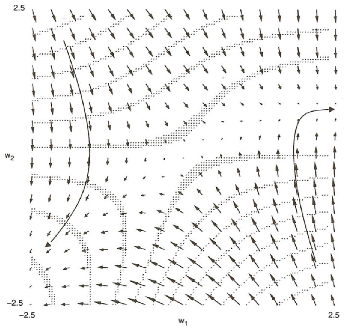
Usually, it is difficult to see why a network has been caught in a local minimum. However, in this very simple case, we have only two weights and can produce a contour map for the error space. The map is shown in Figure 5.12. It is perhaps difficult to visualize, but the map roughly shows a saddle shape. It is high on the upper left and lower right and slopes down toward the center. It then slopes off on each side toward the two minima. If the initial values of the weights begin one part of the space, the system will follow the contours down and to the left into the minimum in which both weights are negative. If, however, the system begins in another part of the space, the system will follow the slope into the upper right quadrant in which both weights are positive. Eventually, the system moves into a gently sloping valley in which the weight from the hidden unit to the output unit is almost constant at about 0.73 and the weight from the input unit to the hidden unit is slowly increasing. It is slowly being sucked into a local minimum. The directed arrows superimposed on the map illustrate thelines of force and illustrate these dynamics. The long arrows represent two trajectories through weightspace for two different starting points.
It is rare that we can create such a simple illustration of the dynamics of weight-spaces and see how clearly local minima come about. However, it is likely that many of our spaces contain these kinds of saddle-shaped error surfaces. Sometimes, as when the biases are free to move, there is a global minimum on either side of the saddle point. In this case, it doesn’t matter which way you move off. At other times, such as in Figure 5.12, the two sides are of different depths. There is no way the system can sense the depth of a minimum from the edge, and once it has slipped in there is no way out. Importantly, however, we find that high-dimensional spaces (with many weights) have relatively few local minima.
Momentum. Our learning procedure requires only that the change in weight be proportional to the weight error derivative. True gradient descent requires that infinitesimal steps be taken. The constant of proportionality, ϵ, is the learning rate in our procedure. The larger this constant, the larger the changes in the weights. The problem with this is that it can lead to steps that overshoot the minimum, resulting in a large increase in error. For practical purposes we choose a learning rate that is as large as possible without leading to oscillation. This offers the most rapid learning. One way to increase the learning rate without leading to oscillation is to modify the back propagation learning rule to include a momentum term. This can be accomplished by the following rule:

where the subscript n indexes the presentation number and α is a constant that determines the effect of past weight changes on the current direction of movement in weight space. This provides a kind of momentum in weight-space that effectively filters out high-frequency variations of the error surface in the weight-space. This is useful in spaces containing long ravines that are characterized by steep walls on both sides of the ravine and a gently sloping floor. Such situations tend to lead to divergent oscillations across the ravine. To prevent these it is necessary to take very small steps, but this causes very slow progress along the ravine. The momentum tends to cancel out the tendency to jump across the ravine and thus allows the effective weight steps to be bigger. In most of the simulations reported in PDP:8, α was about 0.9. Our experience has been that we get the same solutions by setting α = 0 and reducing the size of ϵ, but the system learns much faster overall with larger values of α and ϵ.
Symmetry breaking. Our learning procedure has one more problem that can be readily overcome and this is the problem of symmetry breaking. If all weights start out with equal values and if the solution requires that unequal weights be developed, the system can never learn. This is because error is propagated back through the weights in proportion to the values of the weights. This means that all hidden units connected directly to the output units will get identical error signals, and, since the weight changes depend on the error signals, the weights from those units to the output units must always be the same. The system is starting out at a kind of unstable equilibrium point that keeps the weights equal, but it is higher than some neighboring points on the error surface, and once it moves away to one of these points, it will never return. We counteract this problem by starting the system with small random weights. Under these conditions symmetry problems of this kind do not arise. This can be seen in Figure 5.12. If the system starts at exactly (0,0), there is no pressure for it to move at all and the system will not learn; if it starts virtually anywhere else, it will eventually end up in one minimum or the other.
Weight decay. One additional extension of the back propagation model that we will consider here is the inclusion of weight decay. Weight decay is simply a tendency for weights to be reduced very slightly every time they are updated. If weight-decay is non-zero, then the full equation for the change to each weight becomes the following:

where ω is a positive constant representing the strength of the weight decay. Weight decay can be seen as a procedure for minimizing the total magnitude of the weights, where the magnitude is the sum of the squares of the weights. It should be noted that minimizing the sum of the squares of the weights can be in competition with minimizing the error measure, and so if weight decay is too strong it can often interfere with reaching an acceptable performance criterion.
Learning by pattern or by epoch. The derivation of the back propagation rule presupposes that we are taking the derivative of the error function summed over all patterns. In this case, we might imagine that we would present all patterns and then sum the derivatives before changing the weights. Instead, we can compute the derivatives on each pattern and make the changes to the weights after each pattern rather than after each epoch. Although the former approach can be implemented more efficiently (weight error derivatives for each pattern can be computed in parallel over separate processors, for example) the latter approach may be more plausible from a human or biological learning perspective, where it seems that learning does occur “on line”. Also, if the training set is large, consistent weight error derivatives across patterns can add up and produce a huge overshoot in the change to a connection weight. The bp program allows weight changes after each pattern or after each epoch. In fact, the user may specify the size of a batch of patterns to be processed before weights are updated.3
The bp program implements the back propagation process just described. Networks are assumed to be feedforward only, with no recurrence. An implementation of backpropagation for recurrent networks is described in a later chapter.
The network is specified in terms of a set of pools of units. By convention, pool(1) contains the single bias unit, which is always on. Subsequent pools are declared in an order that corresponds to the feed-forward structure of the network. Since activations at later layers depend on the activations at earlier layers, the activations of units must be processed in correct order, and therefore the order of specification of pools of units is important. Indeed, since deltas at each layer depend on the delta terms from the layers further forward, the backward pass must also be carried out in the correct order. Each pool has a type: it can be an input pool, an output pool, or a hidden pool. There can be more than one input pool and more than one output pool and there can be 0 or more hidden pools. Input pools must all be specified before any other pools and all hidden pools must be specified before any output pools.
Connections among units are specified by projections. Projections may be from any pool to any higher numbered pool; since the bias pool is pool(1) it may project to any other pool, although bias projections to input pools will have no effect since activations of input units are clamped to the value specified by the external input. Projections from a layer to itself are not allowed.
Weights in a projection can be constrainted to be positive or negative. These constraints are imposed both at initialization and after each time the weights are incremented during processing. Two other constraints are imposed only when weights are initialized; these constraints specify either a fixed value to which the weight is initialized, or a random value. For weights that are random, if they are constrained to be positive, they are initialized to a value between 0 and the value of a parameter called wrange; if the weights are constrained to be negative, the initialization value is between -wrange and 0; otherwise, the initialization value is between wrange/2 and -wrange/2. Weights that are constrained to a fixed value are initialized to that value.
The program also allows the user to set an individual learning rate for each projection via a layer-specific lrate parameter. If the value of this layer-specific lrate is unspecified, the network-wide lrate variable is used.
The bp program also makes use of a list of pattern pairs, each pair consisting of a name, an input pattern, and a target pattern. The number of elements in the input pattern should be equal to the total number of units summed across all input pools. Similarly, the number of elements of the target pattern should be equal to the total number of output units summed across all output pools.
Processing of a single pattern occurs as follows: A pattern pair is chosen, and the pattern of activation specified by the input pattern is clamped on the input units; that is, their activations are set to whatever numerical values are specified in the input pattern. These are typically 0’s and 1’s but may take any real value.
Next, activations are computed. For each noninput pool, the net inputs to each unit are computed and then the activations of the units are set. This occurs in the order that the pools are specified in the network specification, which must be specified correctly so that by the time each unit is encountered, the activations of all of the units that feed into it have already been set. The routine performing this computation is called compute_output. Once the output has been computed some summary statistics are computed in a routine called sumstats. First it computes the pattern sum of squares (pss), equal to the squared error terms summed over all of the output units. Analogously, the pce or pattern cross entropy, the sum of the cross entropy terms accross all the output units, is calculated. Then the routine adds the pss to the total sum of squares (tss), which is just the cumulative sum of the pss for all patterns thus far processed within the current epoch. Similarly the pce is added to the tce, or total cross entropy measure.
Next, error and delta terms are computed in a routine called compute_error. The error for a unit is equivalent to (minus) the partial derivative of the error with respect to a change in the activation of the unit. The delta for the unit is (minus) the partial derivative of the error with respect to a change in the net input to the unit. First, the error terms are calculated for each output unit. For these units, error is the difference between the target and the obtained activation of the unit. After the error has been computed for each output unit, we get to the ”heart” of back propagation: the recursive computation of error and delta terms for hidden units. The program iterates backward over the layers, starting with the last output layer. The first thing it does in each layer is set the value of delta for the units in the current layer; this is equal to the error for the unit times the derivative of the activation function as described above. Then, once it has the delta terms for the current pool, the program passes this back to all pools that project to the current pool; this is the actual back propagation process. By the time a particular pool becomes the current pool, all of the units that it projects to will have already been processed and its total error will have been accumulated, so it is ready to have its delta computed.
After the backward pass, the weight error derivatives are then computed from the deltas and activations in a routine called compute_weds. Note that this routine adds the weight error derivatives occasioned by the present pattern into an array where they can potentially be accumulated over patterns.
Weight error derivatives actually lead to changes in the weights when a routine called change_weights is called. This may be called after each pattern has been processed, or after each batch of n patterns, or after all patterns in the training set have been processed. When this routine is called, it cycles through all the projections in the network. For each, the new delta weight is first calculated. The delta weight is equal to (1) the accumulated weight error derivative scaled by the lrate, minus the weight decay scaled by wdecay, plus a fraction of the previous delta weight where the fraction is the value of the momentum parameter. Then, this delta weight is added into the weight, so that the weight’s new value is equal to its old value plus the delta weight. At the end of processing each projection, the weight error derivative terms are all set to 0, and constraints on the values of the weights are imposed in the routine constrain_weights.
Generally, learning is accomplished through a sequence of epochs, in which all pattern pairs are presented for one trial each during each epoch. The presentation is either in sequential or permuted order. It is also possible to test the processing of patterns, either individually or by sequentially cycling through the whole list, with learning turned off. In this case, compute_output, compute_error, and sumstats are called, but compute_wed and change_weights are not called.
The bp program is used much like earlier programs in this series, particularly pa. Like the other programs, it has a flexible architecture that is specified using a .net file, and a flexible screen layout that is specified in a .tem file. The program also makes use of a .pat file, in which the pairs of patterns to be used in training and testing the network are listed.
When networks are initialized, the weights are generally assigned according to a pseudo-random number generator. As in pa and iac, the reset command allows the user to repeat a simulation run with the same initial configuration used just before. (Another procedure for repeating the previous run is described in Ex. 5.1.) The newstart command generates a new random seed and seeds the random number generator with it before using the seed in generating a new set of random initial values for the connection weights.
Control over learning occurs by setting options in the training window or via the settrainopts function. The number of epochs nepochs to train each time “run” is called can be specified. The user can also specify whether weights are updated after every pattern, after n patterns, or after every epoch, and whether the mode of pattern presentation is sequential strain or permuted ptrain. The learning rate, weight decay, and momentum parameters can all be specified as well. The user can also set a stopping criterion for training called “ecrit”. The variable wrange, the range of values allowed when weights are initialized or re-initialized, can also be adjusted.
fast mode for training. The bp program’s inner loops have been converted to fast mex code (c code that interfaces with MATLAB). To turn on the fast mode for network training, click the ’fast’ option in the train window. This option can also be set by typing the following command on the MATLAB command prompt:
runprocess(’process’,’train’,’granularity’,’epoch’,’count’,1,’fastrun’,1);
There are some limitations in executing fast mode of training.In this mode, network output logs can only be written at epoch level. Any smaller output frequency if specified, will be ignored.When running with fast code in gui mode, network viewer will only be updated at epoch level.Smaller granularity of display update is disabled to speed up processing. The ’cascade’ option of building activation gradually is also not available in fast mode.
There is a known issue with running this on linux OS.MATLAB processes running fast version appear to be consuming a lot of system memory. This memory management issue has not been observed on windows. We are currently investigating this and will be updating the documentation as soon as we find a fix.
In the bp program the principle measures of performance are the pattern sum of squares (pss) and the total sum of squares (tss), and the pattern cross-entropy pce and the total cross entropy tce. The user can specify whether the error measure used in computing error derivatives is the sum squared error or the cross entropy. Because of its historical precedence, the sum squared error is used by default. The user may optionally also compute an additional measure, the vector correlation of the present weight error derivatives with the previous weight error derivatives. The set of weight error derivatives can be thought of as a vector pointing in the steepest direction downhill in weight space; that is, it points down the error gradient. Thus, the vector correlation of these derivatives across successive epochs indicates whether the gradient is staying relatively stable or shifting from epoch to epoch. For example, a negative value of this correlation measure (called gcor for gradient correlation) indicates that the gradient is changing in direction. Since the gcor can be thought of as following changes in the direction of the gradient, the check box for turning on this computation is called follow
Control over testing is straightforward. With the “test all” box checked, the user may either click run to carry out a complete pass through the test set, or click step to step pattern by pattern, or the user may uncheck the “text all” button and select an individual pattern by clicking on it in the network viewer window and then clicking run or step.
There is a special mode available in the bp program called cascade mode. This mode allows activation to build up gradually rather than being computed in a single step as is usually the case in bp. A discussion of the implementation and use of this mode is provided later in this chapter.
As with other pdptool programs the user may adjust the frequency of display updating in the train and test windows. It is also possible to log and create graphs of the state of the network at the pattern or epoch level using create/edit logs within the training and testing options panels.
We present four exercises using the basic back propagation procedure. The first one takes you through the XOR problem and is intended to allow you to test and consolidate your basic understanding of the back propagation procedure and the gradient descent process it implements. The second allows you to explore the wide range of different ways in which the XOR problem can be solved; as you will see the solution found varies from run to run initialized with different starting weights. The third exercise suggests minor variations of the basic back propagation procedure, such as whether weights are changed pattern by pattern or epoch by epoch, and also proposes various parameters that may be explored. The fourth exercise suggests other possible problems that you might want to explore using back-propagation.
The XOR problem is described at length in PDP:8. Here we will be considering one of the two network architectures considered there for solving this problem. This architecture is shown in Figure 5.13. In this network configuration there are two input units, one for each “bit” in the input pattern. There are also two hidden units and one output unit. The input units project to the hidden units, and the hidden units project to the output unit; there are no direct connections from the input units to the output units.
All of the relevant files for doing this exercise are contained in the bp directory; they are called xor.tem, xor.net, xor.pat, and xor. wts.
Once you have downloaded the latest version of the software, started MATLAB, set your path to include the pdptool directory and all of its children, and changed to the bp directory, you can simply type
bpxor
to the MATLAB command-line prompt. This file instructs the program to set up the network as specified in the xor.net file and to read the patterns as specified in the xor.pat file; it also initializes various variables. Then it reads in an initial set of weights to use for this exercise. Finally, a test of all of the patterns in the training set is performed. The network viewer window that finally appears shows the state of the network at the end of this initial test of all of the patterns. It is shown in Figure 5.14.
The display area in the network viewer window shows the current epoch number and the total sum of of squares (tss) resulting from testing all four patterns. The next line contains the value of the gcor variable, currently 0 since no error derivatives have yet been calculated. Below that is a line containing the current pattern name and the pattern sum of squares pss associated with this pattern. To the right in the “patterns” panel is the set of input and target patterns for XOR. Back in the main network viewer window, we now turn our attention to the area to the right and below the label “sender acts”. The colored squares in this row shows the activations of units that send their activations forward to other units in the network. The first two are the two input units, and the next two are the two hidden units. Below each set of sender activations are the corresponding projections, first from the input to the hidden units, and below and to the right of that, from the hidden units to the single output unit. The weight in a particular column and row represents the strength of the connection from a particular sender unit indexed by the column to the particular receiver indexed by the row.
To the right of the weights is a column vector indicating the values of the bias terms for the receiver units-that is, all the units that receive input from other units. In this case, the receivers are the two hidden units and the output unit.
To the right of the biases is a column for the net input to each receiving unit. There is also a column for the activations of each of these receiver units. (Note that the hidden units’ activations appear twice, once in the row of senders and once in this column of receivers.) The next column contains the target vector, which in this case has only one element since there is only one output unit. Finally, the last column contains the delta values for the hidden and output units.
Note that shades of red are used to represent positive values, shades of blue are used for negative values, and a neutral gray color is used to represent 0. The color scale for weights, biases, and net inputs ranges over a very broad range, and values less than about .5 are very faint in color. The color scale for activations ranges over somewhat less of a range, since activations can only range from 0 to 1. The color scale for deltas ranges over a very small range since delta values are very small. Even so, the delta values at the hidden level show very faintly compared with those at the output level, indicating just how small these delta values tend to be, at least at this early stage of training. You can inspect the actual numberical values of each variable by moving your mouse over the corresponding colored square.
The display shows what happened when the last pattern pair in the file xor.pat was processed. This pattern pair consists of the input pattern (1 1) and the target pattern (0). This input pattern was clamped on the two input units. This is why they both have activation values of 1.0, shown as a fairly saturated red in the first two entries of the sender activation vector. With these activations of the input units, coupled with the weights from these units to the hidden units, and with the values of the bias terms, the net inputs to the hidden units were set to 0.60 and -0.40, as indicated in the net column. Plugging these values into the logistic function, the activation values of 0.64 and 0.40 were obtained for these units. These values are shown both in the sender activation vector and in the receiver activation vector (labeled act, next to the net input vector). Given these activations for the hidden units, coupled with the weights from the hidden units to the output unit and the bias on the output unit, the net input to the output unit is 0.48, as indicated at the bottom of the net column. This leads to an activation of 0.61, as shown in the last entry of the act column. Since the target is 0.0, as indicated in the target column, the error, or (target - activation) is -0.61; this error, times the derivative of the activation function (that is, activation (1 - activation)) results in a delta value of -0.146, as indicated in the last entry of the final column. The delta values of the hidden units are determined by back propagating this delta term to the hidden units, using the back-propagation equation.
Q.5.1.1.
Show the calculations of the values of delta for each of the two hidden units, using the activations and weights as given in this initial screen display, and the BP Equation. Explain why these values are so small.
At this point, you will notice that the total sum of squares before any learning has occurred is 1.0507. Run another tall to understand more about what is happening.
Q.5.1.2.
Report the output the network produces for each input pattern and explain why the values are all so similar, referring to the strengths of the weights, the logistic function, and the effects of passing activation forward through the hidden units before it reaches the output units.
Now you are ready to begin learning. Acivate the training panel. If you click run (don’t do that yet), this will run 30 epochs of training, presenting each pattern sequentially in the order shown in the patterns window within each epoch, and adjusting the weights at the end of the epoch. If you click step, you can follow the tss and gcor measures as they change from epoch to epoch. A graph will also appear showing the tss. If you click run after clicking step a few times, the network will run to the 30 epoch milestone, then stop.
You may find in the course of running this exercise that you need to go back and start again. To do this, you should use the reset command, followed by clicking on the load weights button, and selecting the file xor.wts. This file contains the initial weights used for this exercise. This method of reinitializing guarantees that all users will get the same starting weights.
After completing the first 30 epochs, stop and answer this question.
Q.5.1.3.
The total sum of squares is smaller at the end of 30 epochs, but is only a little smaller. Describe what has happened to the weights and biases and the resulting effects on the activation of the output units. Note the small sizes of the deltas for the hidden units and explain. Do you expect learning to proceed quickly or slowly from this point? Why?
Run another 90 epochs of training (for a total of 120) and see if your predictions are confirmed. As you go along, watch the progression of the tss in the graph that should be displayed (or keep track of this value at each 30 epoch milestone by recording it manually). You might find it interesting to observe the results of processing each pattern rather than just the last pattern in the four-pattern set. To do this, you can set the update after selection to 1 pattern rather than 1 epoch, and use the step button for an epoch or two at the beginning of each set of 30 epochs.
At the end of another 60 epochs (total: 180), some of the weights in the network have begun to build up. At this point, one of the hidden units is providing a fairly sensitive index of the number of input units that are on. The other is very unresponsive.
Q.5.1.4.
Explain why the more responsive hidden unit will continue to change its incoming weights more rapidly than the other unit over the next few epochs.
Run another 30 epochs. At this point, after a total of 210 epochs, one of the hidden units is now acting rather like an OR unit: its output is about the same for all input patterns in which one or more input units is on.
Q.5.1.5.
Explain this OR unit in terms of its incoming weights and bias term. What is the other unit doing at this point?
Now run another 30 epochs. During these epochs, you will see that the second hidden unit becomes more differentiated in its response.
Q.5.1.6.
Describe what the second hidden unit is doing at this point, and explain why it is leading the network to activate the output unit most strongly when only one of the two input units is on.
Run another 30 epochs. Here you will see the tss drop very quickly.
Q.5.1.7.
Explain the rapid drop in the tss, referring to the forces operating on the second hidden unit and the change in its behavior. Note that the size of the delta for this hidden unit at the end of 270 epochs is about as large in absolute magnitude as the size of the delta for the output unit. Explain.
Click the run button one more time. Before the end of the 30 epochs, the value of tss drops below ecrit, and so training stops. The XOR problem is solved at this point.
Q.5.1.8.
Summarize the course of learning, and compare the final state of the weights with their initial state. Can you give an approximate intuitive account of what has happened? What suggestions might you make for improving performance based on this analysis?
Run the XOR problem several more times, each time using newstart to get a new random configuration of weights. Write down the value of the random seed after each newstart (you will find it by clicking on Set Seed in the upper left hand corner of the network viewer window). Then run for up to 1000 epochs, or until the tss reaches the criterion (you can set nepochs in the test window to 1000, and set update after to, say, 50 epochs). We will call cases in which the tss reaches the criterion successful cases. Continue til you find two successful runs that reach different solutions than the one found in Exercise 5.1. Read on for further details before proceeding.
Q.5.2.1.
At the end of each run, record, after each random seed, the final epoch number, and the final tss. Create a table of these results to turn in as part of your homework. Then, run through a test, inspecting the activations of each hidden unit and the single output unit obtained for each of the four patterns. Choose two successful runs that seem to have reached different solutions than the one reached in Exercise 5.1, as evidenced by qualitative differences in the hidden unit activation patterns. For these two runs, record the hidden and output unit activations for each of the four patterns, and include these results in a second table as part of what you turn in. For each case, state what logical predicate each hidden unit appears to be calculating, and how these predicates are then combined to determine the activation of the output unit. State this in words for each case, and also use the notation described in the hint below to express this information succinctly.
Hint. The question above may seem hard at first, but should become easier as you consider each case. In Excercise 5.1, one hidden unit comes on when either input unit is on (i.e., it acts as an OR unit), and the other comes on when both input units are on (i.e., it acts as an AND unit). For this exercise, we are looking for qualitatively different solutions. You might find that one hidden unit comes on when the first input unit is on and the second is off (This could be called ‘A and not B’), and the other comes on when the first is on and the second is off (‘B and not A’). The weights from the hidden units to the output unit will be different from what they were in Exercise 5.1, reflecting a difference in the way the predicates computed by each hidden unit are combined to solve the XOR problem. In each case you should be able to describe the way the problem is being solved using logical expressions. Use A for input unit 1, B for input unit 2, and express the whole operation as a compound logical statement, using the additional logical terms ’AND’ ’OR’ and ’NOT’. Use square brackets around the expression computed by each hidden unit, then use logical terms to express how the predicates computed by each hidden unit are combined. For example, for the case in Exercise 5.1, we would write: [A OR B] AND NOT [A AND B].
There are several further studies one can do with XOR. You can study the effects of varying:
1. One of the parameters of the model (lrate, wrange, momentum).
2. Frequency of weight updating: once per pattern or epoch.
3. The training regime: permuted vs. sequential presentation. This makes a difference only when the frequency of weight updating is equal to pattern.
4. The magnitude of the initial random weights (determined by wrange,).
5. The error measure: cross-entropy vs. sum squared error.
You are encouraged to do your own exploration of one of these parameters, trying to examine its effects of the rate and outcome of learning. We don’t want to prescribe your experiments too specifically, but one thing you could do would be the following. Re-run each of the eight runs that you carried out in the previous exercise under the variation that you have chosen. To do this, you first set the training option for your chosen variation, then you set the random seed to the value from your first run above, then click reset. The network will now be initialized exactly as it was for that first run, and you can now test the effect of your chosen variation by examining whether it effects the time course or the outcome of learning. You could repeat these steps for each of your runs, exploring how the time course and outcome of learning are affected.
Q.5.3.1.
Describe what you have chosen to vary, how you chose to vary it, and present the results you obtained in terms of the rate of learning, the evolution of the weights, and the eventual solution achieved. Explain as well as you can why the change you made had the effects you found.
For a thorough investigation, you might find it interesting to try several different values along the dimension you have chosen to vary, and see how these parametric variations affect your solutions. Sometimes, in such explorations, you can find that things work best with an intermediate value of some parameter, and get worse for both larger and smaller values.
This exercise encourages you to construct a different problem to study, either choosing from those discussed in PDP:8 or choosing a problem of your own. Set up the appropriate network, template, pattern, and start-up files, and experiment with using back propagation to learn how to solve your problem.
Q.5.4.1.
Describe the problem you have chosen, and why you find it interesting. Explain the network architecture that you have selected for the problem and the set of training patterns that you have used. Describe the results of your learning experiments. Evaluate the back propagation method for learning and explain your feelings as to its adequacy, drawing on the results you have obtained in this experiment and any other observations you have made from the readings or from this exercise.
Hints. To create your own network, you will need to create the necessary .net, .tem, and .pat files yourself; once you’ve done this, you can create a script file (with .m extension) that reads these files and launches your network. The steps you need to take to do this are described in Appendix B, How to create your own network. More details are available in the PDPTool User’s Guide, Appendix C.
In general, if you design your own network, you should strive to keep it simple. You can learn a lot with a network that contains as few as five units (the XOR network considered above), and as networks become larger they become harder to understand.
To achieve success in training your network, there are many parameters that you may want to consider. The exercises above should provide you with some understanding of the importance of some of these parameters. The learning rate (lrate) of your network is important; if it is set either too high or too low, it can hinder learning. The default 0.1 is fine for some simple networks (e.g., the 838 encoder example discussed in Appendix B), but smaller rates such as 0.05, 0.01 or 0.001 are often used, especially in larger networks. Other parameters to consider are momentum, the initial range of the weights (wrange), the weight update frequency variable, and the order of pattern presentation during training (all these are set through the train options window).
If you are having trouble getting your network to learn, the following approach may not lead to the fastest learning but it seems fairly robust: Set momentum to 0, set the learning rate fairly low (.01), set the update frequency to 1 pattern, set the training regime to permuted (ptrain), and use cross-entropy error. If your network still doesn’t learn make sure your network and training patterns are specified correctly. Sometimes, it may also be necessary to add hidden units, though it is surprising how few you can get away with in many cases, though with the minimum number, as we know from XOR, you can get stuck sometimes.
The range of the initial random weights can hinder learning if it is set too high or too low. A range that is too high (such as 20) will push the hidden units to extreme activation values (0 or 1) before the network has started learning, which can harm learning (why?). If this parameter is too small (such as .01), learning can also be very slow since the weights dilute the back propagation of error. The default wrange of 1 is ok for smaller networks, but it may be too big for larger networks. Also, it may be worth noting that, while a smaller wrange and learning rate tends to lead to slower learning, it tends to produce more consistent results across different runs (using different initial random weights).
Other pre-defined bp networks. In addition to XOR, there are two further examples provided in the PDPTool/bp directory. One of these is the 4-2-4 encoder problem described in PDP:8. The files 424.tem, 424.net, 424.pat, and FourTwoFour.m are already set up for this problem just type FourTwoFour at the command prompt to start up this network. The network viewer window is layed out as with XOR, such that the activations of the input and hidden units are shown across the top, and the bias, net input, activations, targets and deltas for the hidden and output units are shown in vertical columns to the right of the two arrays of weights.
Another network that is also ready to run is Rumelhart’s Semantic Network, described in Rumelhart and Todd (1993), Rogers and McClelland (2004) (Chapters 2 and 3), and McClelland and Rogers (2003). The files for this are called semnet.net, semnet.tem, EightThings.pat and semnet.m. The exercise can be started by typing semnet to the command prompt. Details of the simulation are close to those used in McClelland and Rogers (2003). Learning takes on the order of 1000 epochs for all patterns to reach low pss values with the given parameters.