Chapter 6
Competitive Learning

In Chapter 5 we showed that multilayer, nonlinear networks are essential for the solution of many problems. We showed one way, the back propagation of error, that a system can learn appropriate features for the solution of these difficult problems. This represents the basic strategy of pattern association—to search out a representation that will allow the computation of a specified function. There is a second way to find useful internal features: through the use of a regularity detector, a device that discovers useful features based on the stimulus ensemble and some a priori notion of what is important. The competitive learning mechanism described in PDP:5 is one such regularity detector. In this section we describe the basic concept of competitive learning, show how it is implemented in the cl program, describe the basic operations of the program, and give a few exercises designed to familiarize the reader with these ideas.

6.1 SIMPLE COMPETITIVE LEARNING

6.1.1 Background

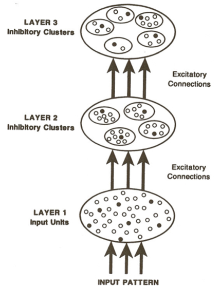
The basic architecture of a competitive learning system (illustrated in Figure 6.1) is a common one. It consists of a set of hierarchically layered units in which each layer connects, via excitatory connections, with the layer immediately above it, and has inhibitory connections to units in its own layer. In the most general case, each unit in a layer receives an input from each unit in the layer immediately below it and projects to each unit in the layer immediately above it. Moreover, within a layer, the units are broken into a set of inhibitory clusters in which all elements within a cluster inhibit all other elements in the cluster. Thus the elements within a cluster at one level compete with one another to respond to the pattern appearing on the layer below. The more strongly any particular unit responds to an incoming stimulus, the more it shuts down the other members of its cluster.

There are many variants to the basic competitive learning model. von der Malsburg (1973), Fukushima (1975), and Grossberg (1976), among others, have developed competitive learning models. In this section we describe the simplest of the many variations. The version we describe was first proposed by Grossberg (1976) and is the one studied by Rumelhart and Zipser (also in PDP:5). This version of competitive learning has the following properties:

• The units in a given layer are broken into several sets of nonoverlapping clusters. Each unit within a cluster inhibits every other unit within a cluster. Within each cluster, the unit receiving the largest input achieves its maximum value while all other units in the cluster are pushed to their minimum value.¹ We have arbitrarily set the maximum value to 1 and the minimum value to 0.
• Every unit in every cluster receives inputs from all members of the same set of input units.
• A unit learns if and only if it wins the competition with other units in its cluster.
• A stimulus pattern S_j consists of a binary pattern in which each element of the pattern is either active or inactive. An active element is assigned the value 1 and an inactive element is assigned the value 0.
• Each unit has a fixed amount of weight (all weights are positive) that is distributed among its input lines. The weight on the line connecting to unit i on the upper layer from unit j on the lower layer is designated w_ij. The fixed total amount of weight for unit j is designated ∑ _jw_ij = 1. A unit learns by shifting weight from its inactive to its active input lines. If a unit does not respond to a particular pattern, no learning takes place in that unit. If a unit wins the competition, then each of its input lines gives up some portion ϵ of its weight and that weight is then distributed equally among the active input lines. Mathematically, this learning rule can be stated

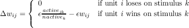  (6.1)

  where active_jk is equal to 1 if in stimulus pattern S_k, unit j in the lower layer is active and is zero otherwise, and nactive_k is the number of active units in pattern S_k (thus nactive_k = ∑ _jactive_jk).²

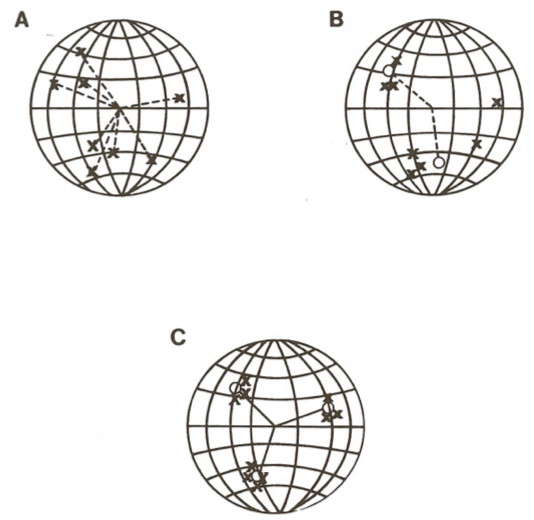
Figure 6.2 illustrates a useful geometric analogy to this system. We can consider each stimulus pattern as a vector. If all patterns contain the same number of active lines, then all vectors are the same length and each can be viewed as a point on an N-dimensional hypersphere, where N is the number of units in the lower level, and therefore, also the number of input lines received by each unit in the upper level. Each × in Figure 6.2A represents a particular pattern. Those patterns that are very similar are near one another on the sphere, and those that are very different are far from one another on the sphere. Note that since there are N input lines to each unit in the upper layer, its weights can also be considered a vector in N-dimensional space. Since all units have the same total quantity of weight, we have N-dimensional vectors of approximately fixed length for each unit in the cluster.³ Thus, properly scaled, the weights themselves form a set of vectors that (approximately) fall on the surface of the same hypersphere. In Figure 6.2B, the ○’s represent the weights of two units superimposed on the same sphere with the stimulus patterns. Whenever a stimulus pattern is presented, the unit that responds most strongly is simply the one whose weight vector is nearest that for the stimulus. The learning rule specifies that whenever a unit wins a competition for a stimulus pattern, it moves a fraction ϵ of the way from its current location toward the location of the stimulus pattern on the hypersphere. Suppose that the input patterns fell into some number, M, of “natural” groupings. Further, suppose that an inhibitory cluster receiving inputs from these stimuli contained exactly M units (as in Figure 6.2C). After sufficient training, and assuming that the stimulus groupings are sufficiently distinct, we expect to find one of the vectors for the M units placed roughly in the center of each of the stimulus groupings. In this case, the units have come to detect the grouping to which the input patterns belong. In this sense, they have “discovered” the structure of the input pattern sets.

6.1.2 Some Features of Competitive Learning

There are several characteristics of a competitive learning mechanism that make it an interesting candidate for study, for example:

• Each cluster classifies the stimulus set into M groups, one for each unit in the cluster. Each of the units captures roughly an equal number of stimulus patterns. It is possible to consider a cluster as forming an M-valued feature in which every stimulus pattern is classified as having exactly one of the M possible values of this feature. Thus, a cluster containing two units acts as a binary feature detector. One element of the cluster responds when a particular feature is present in the stimulus pattern, otherwise the other element responds.
• If there is structure in the stimulus patterns, the units will break up the patterns along structurally relevant lines. Roughly speaking, this means that the system will find clusters if they are there.
• If the stimuli are highly structured, the classifications are highly stable. If the stimuli are less well structured, the classifications are more variable, and a given stimulus pattern will be responded to first by one and then by another member of the cluster. In our experiments, we started the weight vectors in random directions and presented the stimuli randomly. In this case, there is rapid movement as the system reaches a relatively stable configuration (such as one with a unit roughly in the center of each cluster of stimulus patterns). These configurations can be more or less stable. For example, if the stimulus points do not actually fall into nice clusters, then the configurations will be relatively unstable and the presentation of each stimulus will modify the pattern of responding so that the system will undergo continual evolution. On the other hand, if the stimulus patterns fall rather nicely into clusters, then the system will become very stable in the sense that the same units will always respond to the same stimuli.⁴
• The particular grouping done by a particular cluster depends on the starting value of the weights and the sequence of stimulus patterns actually presented. A large number of clusters, each receiving inputs from the same input lines can, in general, classify the inputs into a large number of different groupings or, alternatively, discover a variety of independent features present in the stimulus population. This can provide a kind of distributed representation of the stimulus patterns.
• To a first approximation, the system develops clusters that minimize within-cluster distance, maximize between-cluster distance, and balance the number of patterns captured by each cluster. In general, tradeoffs must be made among these various forces and the system selects one of these tradeoffs.

6.1.3 Implementation

The competitive learning model is implemented in the cl program. The model implements a single input (or lower level) layer of units, each connected to all members of a single output (or upper level) layer of units. The basic strategy for the cl program is the same as for bp and the other learning programs. Learning occurs as follows: A pattern is chosen and the pattern of activation specified by the input pattern is clamped on the input units. Next, the net input into each of the output units is computed. The output unit with the largest input is determined to be the winner and its activation value is set to 1. All other units have their activation values set to 0. The routine that carries out this computation is

After the activation values are determined for each of the output units, the weights must be adjusted according to the learning rule. This involves increasing the weights from the active input lines to the winner and decreasing the weights from the inactive lines to the winner. This routine assumes that each input pattern sums to 1.0 across units, keeping the total amount of weight equal to 1.0 for a given output unit. If we do not want to make this assumption, the routine could easily be modified by implementing Equation 6.1 instead.

6.1.4 Overview of Exercises

We provide an exercise for the cl program. It uses the Jets and Sharks data base to explore the basic characteristics of competitive learning.

Ex6.1. Clustering the Jets and Sharks

The Jets and Sharks data base provides a useful context for studying the clustering features of competitive learning. There are two scripts, jets2 and jets3, where the 2 or 3 in the name indicates that the network has an output cluster of 2 or 3 units. The file jets.pat contains the feature specifications for the 27 gang members. The pattern file is set up as follows: The first column contains the name of each individual. The next two tell whether the individual is a Shark or a Jet, the next three columns correspond to the age of the individual, and so on. Note that there are no inputs corresponding to name units; the name only serves as a label for the convenience of the user. To run the program type

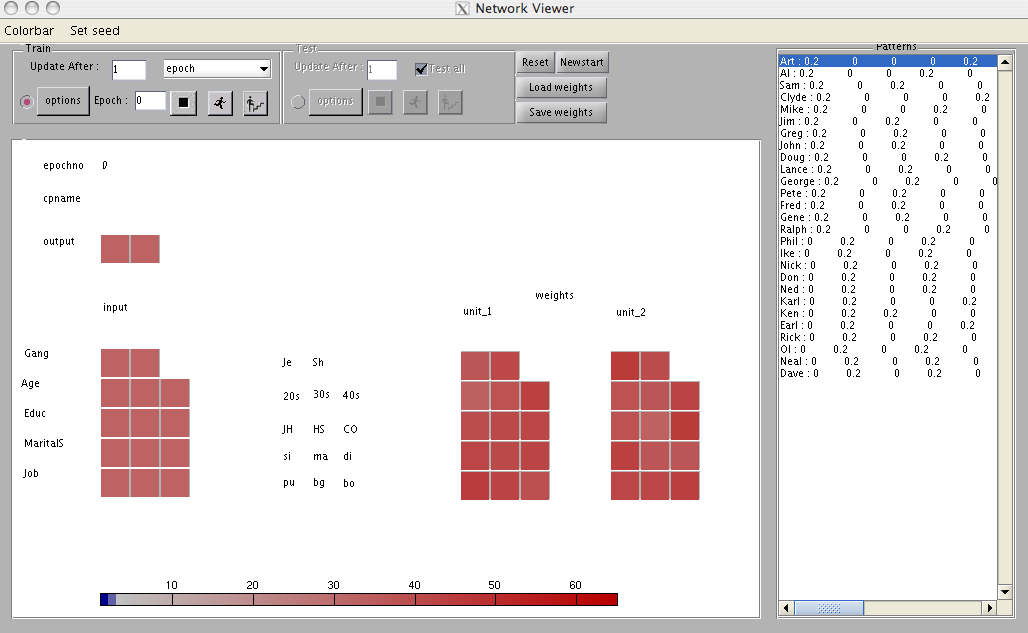
The resulting screen display (shown in Figure 6.3) shows the epoch number, the name of the current pattern, the output vector, the inputs, and the weights from the input units to each of the output units. Between the inputs and the weights is a display indicating the labels of each feature.

The inputs and weights are configured in a manner that mirrors the structure of the features. In this case, the pattern for Art is the current pattern, and patterns sum to 1 across the input units. The first row of inputs indicate the gang to which the individual belongs. In the case of Art, we have a .2 on the left and a 0 on the right. This represents the fact that Art is a Jet and not a Shark. Note that there is at most one .2 in each row. This results from the fact that the values on the various dimensions are mutually exclusive. Art has a .2 for the third value of the Age row, indicating that Art is in his 40s. The rest of the values are similarly interpreted. The weights are in the same configuration as the inputs. The corresponding weight value is displayed below each of the two output unit labels (unit_1 and unit_2). Each cell contains the weight from the corresponding input unit to that output unit. Thus the upper left-hand value for the weights is the initial weight from the Jet unit to output unit 1. Similarly, the lower right-hand value of the weight matrix is the initial weight from bookie to unit 2. The initial values of the weights are random, with the constraint that the weights for each unit sum to 1.0. (Due to scaling and roundoff, the actual values displayed should sum to a value somewhat less than 1.0.) The lrate parameter is set to 0.05. This means that on any trial 5% of the winner’s weight is redistributed to the active lines.

Now try running the program by clicking the run button in the train window. Since nepochs is set to 20, the system will stop after 20 epochs. Look at the new values of the weights. Try several more runs, using the newstart command to reinitialize the system each time. In each case, note the configuration of the weights. You should find that usually one unit gets about 20% of its weight on the jets line and none on the sharks line, while the other unit shows the opposite pattern.

Q.6.1.1.

Hint.

Q.6.1.2.

Now repeat the problem and run it several more times until it reaches a rather different weight configuration. (This may take several tries.) You might be able to find such a state faster by reducing lrate to a smaller value, perhaps 0.02.

Q.6.1.3.

We have prepared a pattern file, called ajets.pat, in which we have deleted explicit information about which gang the individuals represent. Load this file by going to Train options / Pattern file and clicking “Load new.” The same should be done for Test options.

Q.6.1.4.

Thus far the system has used two output units and it therefore classified the patterns into two classes. We have prepared a version with three output units. First, close the pdptool windows. Then access the program by the command:

Q.6.1.5.

6.2 SELF-ORGANIZING MAP

A simple modification to the competitive learning model gives rise to a powerful new class of models: the Self-Organizing Map (SOM). These models were pioneered by Kohonen (1982) and are also referred to as Kohonen Maps.

The SOM can be thought of as the simple competitive learning model with a neighborhood constraint on the output units. The output units are arranged in a spatial grid; for instance, 100 output units might form a 10x10 square grid. Sticking with the hypersphere analogy (Figure 6.2), instead of just moving the winning output unit weights towards the input pattern, the winning unit and its neighbors in the grid are adjusted. The amount of adjustment is determined by the distance in the grid of a given output unit from the winning unit. The effect of this constraint is that neighboring output units tend to respond to similar input pattern, producing a topology preserving map (also called a topographic map) from input space to the output space. This property can be used to visualize structure in high-dimensional input data.

6.2.1 The Model

In terms of the architecture illustrated in Figure 6.1, the SOM model presented here is a layer of input units feeding to a single inhibitory output cluster. Each input unit has a weighted connection to each output unit. However, both the input units and the output units are arranged in two-dimensional grids, adding spatial structure to the network.

Activation of the outputs units is calculated in the much the same way as the simple competitive learning model, with the addition of the winner’s spread of activation to neighbors. First, the net input to each output unit is calculated, and the unit with the largest net input is selected as the winner. The activations of the units are then set according to the Gaussian in Equation 6.2.⁵

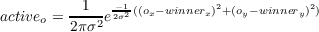(6.2)

where o_x and o_y are the grid x and y coordinates of output unit o and σ² is a spread parameter. The larger the spread, the further learning spreads to the neighbors of the winning unit. The total amount of learning remains approximately constant for different values of σ², which generally starts off larger and is reduced so that global order of the map can be established early during learning.

In contrast to simple competitive learning, all of the network weights are updated for a given input pattern. The weight w_ij to output unit i is updated according to Equation 6.3.

(6.3)

Thus as with simple competitive learning, the output weights are pulled towards the input pattern. This pull is proportional to the activation of the particular output unit and the learning rate ϵ.

6.2.2 Some Features of the SOM

• The simple competitive learning algorithm at the beginning of the chapter was described to cluster input patterns along structurally relevant lines. If there are clusters in the input patterns, the algorithm will usually find them. Also, to a first approximation, the algorithm develops clusters that minimize within-cluster distance, maximize between-cluster distance, and balance the number of patterns captured by each cluster — striking some form of tradeoff between these constraints. The SOM still tries to satisfy these constraints, along with the additional constraint that neighboring output units should cluster similar types of inputs. Thus, the structure found by the map not only reflects input clusters but also attempts to preserve the topology of those clusters.
• In the SOM presented, the net input for an output unit is the inner product of the input vector and the weight vector, as is common for neural networks. This type of model is discussed in Hertz et al. (1991). However, SOMs usually use Euclidean distance between the vectors instead. In this case, the winning output unit would have the smallest distance from the input pattern instead of the largest inner product.
• Hertz et al. (1991) provide a useful analogy, describing the SOM as an “elastic net in input space that wants to come as close as possible to the inputs; the net has the topology of the output array... and the points of the net have the weights as coordinates.”

  To illustrate this point, a simple simulation was run using the Euclidean distance version of the SOM. Input patterns were two dimensional, drawn equally often from one of two circular Gaussians. There was a 5x5 grid of output units, with the weights initialized randomly in a tangled mess (Figure 6.4A). After 250 input patterns, the network dragged the output units towards the patterns, but the network was still a bit tangled and did not span the input space well (Figure 6.4B). After 1000 input patterns, the network spread out to cover more of the patterns, partitioning the output units over the two Gaussians (Figure 6.4C). The “elastic net” was evidently stretched in the middle, since inputs in this region were very sparse.

6.2.3 Implementation

The SOM is also implemented in the cl program. Learning is very similar to simple competitive learning. A pattern is chosen and clamped onto the input units. Using the same routine as simple competitive learning, the output unit with the largest net input is chosen as the winner. Unique to the SOM, the activation of each output unit is set according to the Gaussian function based on distance from the winner. The routine that carries out this computation is:

After the activation values are determined for each of the units, the weights are updated. In contrast with simple competitive learning, not just the winner’s weights are updated. Each of the output units is pulled towards the input pattern in proportion to its activation and the learning rate. This is done with the following routine:

6.2.4 Overview of Exercises

We provide an exercise with the SOM in the cl program, showing how the SOM could be applied as a model of topographic maps in the brain and illustrating some of the basic properties of SOMs.

Ex6.2. Modeling Hand Representation

There are important topology preserving maps in the brain, such as the map between the skin surface and the somatosensory cortex. Stimulating neighboring areas on the skin activate neighboring areas in the cortex, providing a potential application of the SOM model. In this exercise, we apply the SOM to this mapping, inspired by Merzenich’s studies of hand representation. Jenkins et al. (1990) studied reorganization of this mapping (between skin surface and cortex) due to excessive stimulation. Monkeys were trained to repeatedly place their fingertips on a spinning, grooved wheel in order to receive food pellets. After many days of such stimulation, Jenkins et al. found enlargement of the cortical representation of the stimulated skin areas. Inspired by this result, a simulation was set up in which:

• Initially quite random (although biased) projections would be organized by experience to create a smooth and orderly topographic map.
• Concentrating exposure in one part of input space, while receiving input deprivation in another part of space, would lead to re-organization of the map. Presumably, the representation will expand in areas of concentrated input.

To run the software:

1. Start MATLAB, make sure the pdptool path is set, and change to the pdptool/cl directory.
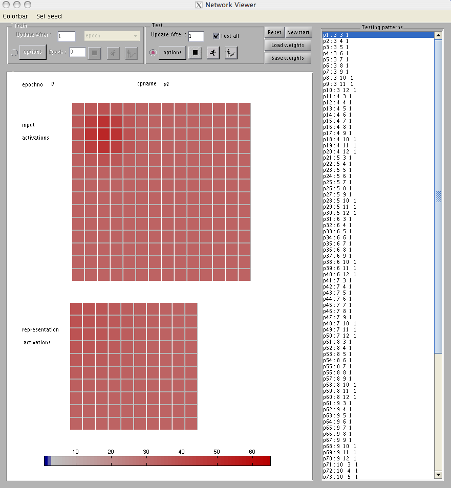
2. At the Matlab prompt, type “topo.” This will bring up two square arrays of units, the upper one representing an input layer (like the skin surface) and the lower one representing an internal representation (like the cortical sheet) This window is displayed in Figure 6.5.
3. Start by running a test to get your bearings. Note that there are training and testing windows, train on the left and testing on the right. To test, click the selector button next to ‘options’ under test. Then select test all (so that it is checked) and click run.

The program will step through 100 input patterns, each producing a blob of activity at a point in the input space. The edges of the input space are used only for the flanks of the blobs, their centers are restricted to a region of 10x10 units. The centers of the blobs will progress across the screen from left to right, then down one row and across again, etc. In the representation layer you will see a large blob of activity that will jump around from point to point based on the relatively random initial weights (more on this in Part 3).

Note that the input patterns are specified in the pattern file with a name, the letter x, then three numerical entries. The first is the x position on the input grid (pat_x), the second is the y position (pat_y), and the third is a spread parameter (σ), determining the width (standard deviation) of the Gaussian blob. All spreads have been set to 1. The activation of an input unit i, at grid coordinates (i_x,i_y), is determined by:

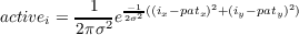(6.4)

which is the same Gaussian function (Equation 6.2) that determines the output activations, depending on the winning unit’s grid position.

The pool structure of the network is as follows:

There is only one projection in the network, net.pool(3).proj(1), which contains the weights in the network.

Part 1: Training the Network

Now you are ready to try to train the network. First, type “net.pool(3).lrange = 2.8” in the Command Window, to set the output activation spread to be initially wide.

To begin training, select the training panel (click the button next to options under train). The network is set up to run 200 epochs of training, with a learning rate (lrate) of .1. The “ptrain” mode is set, meaning that you will be training the network with the patterns presented in a randomly permuted order within each epoch (each pattern is presented once per epoch). The display will update once per epoch, showing the last pattern presented in the epoch in the display. You can reduce the frequency of updating if you like to, say, once per 10 or 20 epochs in the update after window.

Now if you test again, you may see some order beginning to emerge. That is, as the input blob progresses across and then down when you run a test all, the activation blob will also follow the same course. It will probably be jerky and coarse at the point, and sometimes the map comes out twisted. If it is twisted at this stage it is probably stuck.

If it is not twisted, you can proceed to refining the map. This is done by a process akin to annealing, in which you gradually reduce the lrange variable. A reasonable choice reducing it every 200 epochs of training in the following increments: 2.8 for the first 200 epochs, 2.1 for the second 200 epochs, 1.4 for the third 200 epochs, and 0.7 for the last 200 epochs. So, you’ve trained for 200 epochs as lrange = 2.8, so set “net.pool(3).lrange = 2.1.”

Then, run 200 more epochs (just click run) and test again. At this stage the network seems to favor the edges too much (a problem that lessens but often remains throughout the rest of training). Then set net.pool(3).lrange to 1.4 at the command prompt; then run another 200 epochs, then test again, then set it to 0.7, run another 200, then finally test again.

You may or may not have a nice orderly net at this stage. To get a sense of how orderly, you can log your output in the following manner. In test options, click “write output” then “set write options.” Click “start new log” and use the name “part1_log.mat.” Click “Save” and you will return to the set write output panel. In this panel, go into network variables, click net, it will open, click pool(3), it will open, click “winner” in pool(3), then click “add.” The line “pool(3).winner” will then appear under selected. Click “OK.” NOTE: you must also click OK on the Testing options popup for the log to actually be opened for use.

Now run a test again. The results will be logged as a vector showing the winners for each of the 100 input patterns. At the matlab command window you can now load this information into matlab:

Then if you type (without forgetting the transpose operator ’):

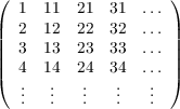
you will get a 10x10 array of the integer indexes of the winners in your command window. The numbers in the array correspond to the winning output unit. The output unit array (the array of colored squares you see on the gui) is column major, meaning that you count vertically 1-10 first and then 11 starts from the next column, so that 1, 11, 21, 31, 41 etc. are on the same horizontal line. In the matrix printed in your command window, the spatial position corresponds to position of the test pattern centers. Thus, a perfect map will be numbered down then across such that it would have 1-10 in the first column, 11-21 in the second column, etc.

** The above array is your first result. Bring this (in printed form) to class for discussion. If your results are not perfect, which is quite likely, what is “wrong” with yours?

NOTE: The log currently stays open and logs all subsequent tests until you shut it off. To do this, click “test options” / “set write options” / and the click “log status off.” You should probably start a new log file each time you want to examine the results, since the contents of the log file will require parsing otherwise. Also the file will then be available to reload and you can examine its contents easily.

Part 2: Changing the seed

The results depend, as in the necker cube, on the value of the random seed. Try the network again with a seed that works pretty well. Go to the very top left of the network viewer, click “set seed,” enter “211579,” then click ok. Then in the upper right find “Reset” and click that. Just setting the seed does not reset the weights. You must click “Reset.” Note that “Reset” resets the system without changing the seed; if you click “Newstart” you will get a different seed.

To save time during training, we have provided a script to automate the process of reducing the lrange parameter. It is provided in “auto_som.m,” and is run by typing “auto_som” in the command prompt.

After training, save your weights after training, for the purposes of Part 4. To do this, click on the “Save weights” button in the upper right of the window. You will load these weights later in this exercise, so remember the folder and name you chose.

After training, the results should be pretty good. Go through the logging steps above, call your log file “part2_log.mat,” and display your results.

**The above array is your second result. Bring this also to class for discussion.

Part 3: Topographic bias in the initial weights

The neighborhood function causes the winning output unit and its neighbors to move their weights in the same direction, developing the property that neighboring output units respond to similar stimuli. However, for the input grid to align properly with the output grid, there must be some underlying topographic bias in the initial weights. Otherwise, the neighborhood function might help create an orderly response grid, but rotated 90 degrees, twisted, or perhaps worse, a jumbled mess. We will explore this initial topographic weight bias in this exercise.

Note that when the network is initialized, the weights are assigned according to the explanation below:

Note that if topbias is 0 there is no topographic bias at all in the initial weights, and the weights are random. On the other hand if topbias is 1 the weights are pre-initialized to have a clear topographic (Gaussian) shape, governed by standard deviation “ispread” (stands for “initial spread of weights”). These parameters are associated with net.pool(3).proj(1), and their values are:

Q.6.2.1.

Q.6.2.2.

** Bring these printed answers to class.

Part 4: Map reorganization through modified stimulation

The purpose of Part 4 is to demonstrate that after the map reaches a reasonable and stable organization, the map can be reorganized given a different distribution of inputs, like the monkey finger tips in Jenkins et al. (1990), with expanded representation in areas of high stimulation.

In this final part of the homework, a developed map will be selectively stimulated in the bottom half of the input space, receiving no input in the upper half. This, of course, is not analogous to the experiment, since the monkeys would also receive stimulation in other areas of the hand not in contact with the wheel. This exercise is rather a simplification to suggest how reorganization is possible in the SOM.

First, load the weights for the trained network that you saved in Part 2. Do this by clicking the Load weights button and select your saved weights. After the weights are loaded, do a test cycle to ensure that the map is already trained.

After this, go into training options. Where it says Pattern file: Click “Load new.” Select “topo_half.pat.” In case you want to switch the patterns back, topo.pat is the standard pattern file that you have been using.

Set net.pool(3).lrange = 0.7, and train the network for 400 epochs. After training, test the network. Changing the patterns before only applies to the training set, and you will want to change the test patterns as well. Thus, go to test options, and click “Load New,” and select topo_half.pat. Also, start a new test log as described in Part 1 and create the log “part4_log.mat.” Test the patterns and observe how the network now responds to this selected set of lower-half test patterns. Then type (without forgetting the transpose operator after the second line):

This grid corresponds to only the winners for the bottom 50 input patterns. The first row was most telling of the reorganization. Compare it with the 6th row of your saved array from Part 2. The perfect map in Part 2 would have this row numbered 6, 16, 26, …, 96. If the ones digits in the row are numbers other than 6, this would be indicative of reorganization. Specifically, if the ones digits are 4 or 5, that means the representation of this input row has creeped upwards, taking over territory that would previously have responded to the upper half of the patterns.

** This array is your third result. Bring this also to class for discussion.

NOTE: You can either test with the same patterns you train with, or with the original set of 100 patterns. The program generally allows different sets of patterns for training and testing.