Chapter 2
Interactive Activation and Competition

Our own explorations of parallel distributed processing began with the use of interactive activation and competition mechanisms of the kind we will examine in this chapter. We have used these kinds of mechanisms to model visual word recognition (McClelland and Rumelhart, 1981; Rumelhart and McClelland, 1982) and to model the retrieval of general and specific information from stored knowledge of individual exemplars (McClelland, 1981), as described in PDP:1. In this chapter, we describe some of the basic mathematical observations behind these mechanisms, and then we introduce the reader to a specific model that implements the retrieval of general and specific information using the “Jets and Sharks” example discussed in PDP:1 (pp. 25-31).

After describing the specific model, we will introduce the program in which this model is implemented: the iac program (for interactive activation and competition). The description of how to use this program will be quite extensive; it is intended to serve as a general introduction to the entire package of programs since the user interface and most of the commands and auxiliary files are common to all of the programs. After describing how to use the program, we will present several exercises, including an opportunity to work with the Jets and Sharks example and an opportunity to explore an interesting variant of the basic model, based on dynamical assumptions used by Grossberg (e.g., (Grossberg, 1978)).

2.1 BACKGROUND

The study of interactive activation and competition mechanisms has a long history. They have been extensively studied by Grossberg. A useful introduction to the mathematics of such systems is provided in Grossberg (1978). Related mechanisms have been studied by a number of other investigators, including Levin (1976), whose work was instrumental in launching our exploration of PDP mechanisms.

An interactive activation and competition network (hereafter, IAC network) consists of a collection of processing units organized into some number of competitive pools. There are excitatory connections among units in different pools and inhibitory connections among units within the same pool. The excitatory connections between pools are generally bidirectional, thereby making the processing interactive in the sense that processing in each pool both influences and is influenced by processing in other pools. Within a pool, the inhibitory connections are usually assumed to run from each unit in the pool to every other unit in the pool. This implements a kind of competition among the units such that the unit or units in the pool that receive the strongest activation tend to drive down the activation of the other units.

The units in an IAC network take on continuous activation values between a maximum and minimum value, though their output—the signal that they transmit to other units—is not necessarily identical to their activation. In our work, we have tended to set the output of each unit to the activation of the unit minus the threshold as long as the difference is positive; when the activation falls below threshold, the output is set to 0. Without loss of generality, we can set the threshold to 0; we will follow this practice throughout the rest of this chapter. A number of other output functions are possible; Grossberg (1978) describes a number of other possibilities and considers their various merits.

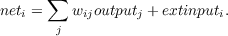
The activations of the units in an IAC network evolve gradually over time. In the mathematical idealization of this class of models, we think of the activation process as completely continuous, though in the simulation modeling we approximate this ideal by breaking time up into a sequence of discrete steps. Units in an IAC network change their activation based on a function that takes into account both the current activation of the unit and the net input to the unit from other units or from outside the network. The net input to a particular unit (say, unit i) is the same in almost all the models described in this volume: it is simply the sum of the influences of all of the other units in the network plus any external input from outside the network. The influence of some other unit (say, unit j) is just the product of that unit’s output, output_j, times the strength or weight of the connection to unit i from unit j. Thus the net input to unit i is given by

(2.1)

In the IAC model, output_j = [a_j]⁺. Here, a_j refers to the activation of unit j, and the expression [a_j]⁺ has value a_j for all a_j > 0; otherwise its value is 0. The index j ranges over all of the units with connections to unit i. In general the weights can be positive or negative, for excitatory or inhibitory connections, respectively.

Human behavior is highly variable and IAC models as described thus far are completely deterministic. In some IAC models, such as the interactive activation model of letter perception (McClelland and Rumelhart, 1981) these deterministic activation values are mapped to probabilities. However, it became clear in detailed attempts to fit this model to data that intrinsic variability in processing and/or variability in the input to a network from trial to trial provided better mechanisms for allowing the models to provide detailed fits to data. McClelland (1991) found that injecting normally distributed random noise into the net input to each unit on each time cycle allowed such networks to fit experimental data from experiments on the joint effects of context and stimulus information on phoneme or letter perception. Including this in the equation above, we have:

(2.2)

Where normal(0,noise) is a sample chosen from the standard normal distribution with mean 0 and standard deviation of noise. For simplicity, noise is set to zero in many IAC network models.

Once the net input to a unit has been computed, the resulting change in the activation of the unit is as follows:

If (net_i > 0),

Otherwise,

Note that in this equation, max, min, rest, and decay are all parameters. In general, we choose max = 1, min ≤ rest ≤ 0, and decay between 0 and 1. Note also that a_i is assumed to start, and to stay, within the interval [min,max].

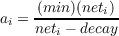
Suppose we imagine the input to a unit remains fixed and examine what will happen across time in the equation for Δa_i. For specificity, let’s just suppose the net input has some fixed, positive value. Then we can see that Δa_i will get smaller and smaller as the activation of the unit gets greater and greater. For some values of the unit’s activation, Δa_i will actually be negative. In particular, suppose that the unit’s activation is equal to the resting level. Then Δa_i is simply (max - rest)net_i. Now suppose that the unit’s activation is equal to max, its maximum activation level. Then Δa_i is simply (-decay)(max - rest). Between these extremes there is an equilibrium value of a_i at which Δa_i is 0. We can find what the equilibrium value is by setting Δa_i to 0 and solving for a_i:

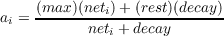(2.3)

Using max = 1 and rest = 0, this simplifies to

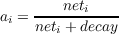(2.4)

What the equation indicates, then, is that the activation of the unit will reach equilibrium when its value becomes equal to the ratio of the net input divided by the net input plus the decay. Note that in a system where the activations of other units—and thus of the net input to any particular unit—are also continually changing, there is no guarantee that activations will ever completely stabilize—although in practice, as we shall see, they often seem to.

Equation 3 indicates that the equilibrium activation of a unit will always increase as the net input increases; however, it can never exceed 1 (or, in the general case, max) as the net input grows very large. Thus, max is indeed the upper bound on the activation of the unit. For small values of the net input, the equation is approximately linear since x∕(x + c) is approximately equal to x∕c for x small enough.

We can see the decay term in Equation 3 as acting as a kind of restoring force that tends to bring the activation of the unit back to 0 (or to rest, in the general case). The larger the value of the decay term, the stronger this force is, and therefore the lower the activation level will be at which the activation of the unit will reach equilibrium. Indeed, we can see the decay term as scaling the net input if we rewrite the equation as

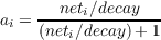(2.5)

When the net input is equal to the decay, the activation of the unit is 0.5 (in the general case, the value is (max + rest)∕2). Because of this, we generally scale the net inputs to the units by a strength constant that is equal to the decay. Increasing the value of this strength parameter or decreasing the value of the decay increases the equilibrium activation of the unit.

In the case where the net input is negative, we get entirely analogous results:

(2.6)

Using rest = 0, this simplifies to

(2.7)

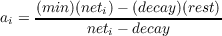
This equation is a bit confusing because net_i and min are both negative quantities. It becomes somewhat clearer if we use amin (the absolute value of min) and anet_i (the absolute value of net_i). Then we have

(2.8)

What this last equation brings out is that the equilibrium activation value obtained for a negative net input is scaled by the magnitude of the minimum (amin). Inhibition both acts more quickly and drives activation to a lower final level when min is farther below 0.

2.1.1 How Competition Works

So far we have been considering situations in which the net input to a unit is fixed and activation evolves to a fixed or stable point. The interactive activation and competition process, however, is more complicated than this because the net input to a unit changes as the unit and other units in the same pool simultaneously respond to their net inputs. One effect of this is to amplify differences in the net inputs of units. Consider two units a and b that are mutually inhibitory, and imagine that both are receiving some excitatory input from outside but that the excitatory input to a (e_a) is stronger than the excitatory input to b (e_b). Let γ represent the strength of the inhibition each unit exerts on the other. Then the net input to a is

(2.9)

and the net input to b is

(2.10)

As long as the activations stay positive, output_i = a_i, so we get

(2.11)

and

(2.12)

From these equations we can easily see that b will tend to be at a disadvantage since the stronger excitation to a will tend to give a a larger initial activation, thereby allowing it to inhibit b more than b inhibits a. The end result is a phenomenon that Grossberg (1976) has called “the rich get richer” effect: Units with slight initial advantages, in terms of their external inputs, amplify this advantage over their competitors.

2.1.2 Resonance

Another effect of the interactive activation process has been called “resonance” by Grossberg (1978). If unit a and unit b have mutually excitatory connections, then once one of the units becomes active, they will tend to keep each other active. Activations of units that enter into such mutually excitatory interactions are therefore sustained by the network, or “resonate” within it, just as certain frequencies resonate in a sound chamber. In a network model, depending on parameters, the resonance can sometimes be strong enough to overcome the effects of decay. For example, suppose that two units, a and b, have bidirectional, excitatory connections with strengths of 2 x decay . Suppose that we set each unit’s activation at 0.5 and then remove all external input and see what happens. The activations will stay at 0.5 indefinitely because

Thus, IAC networks can use the mutually excitatory connections between units in different pools to sustain certain input patterns that would otherwise decay away rapidly in the absence of continuing input. The interactive activation process can also activate units that were not activated directly by external input. We will explore these effects more fully in the exercises that are given later.

2.1.3 Hysteresis and Blocking

Before we finish this consideration of the mathematical background of interactive activation and competition systems, it is worth pointing out that the rate of evolution towards the eventual equilibrium reached by an IAC network, and even the state that is reached, is affected by initial conditions. Thus if at time 0 we force a particular unit to be on, this can have the effect of slowing the activation of other units. In extreme cases, forcing a unit to be on can totally block others from becoming activated at all. For example, suppose we have two units, a and b, that are mutually inhibitory, with inhibition parameter gamma equal to 2 times the strength of the decay, and suppose we set the activation of one of these units—unit a—to 0.5. Then the net input to the other—unit b—at this point will be (-0.5) (2) (decay) = -decay. If we then supply external excitatory input to the two units with strength equal to the decay, this will maintain the activation of unit a at 0.5 and will fail to excite b since its net input will be 0. The external input to b is thereby blocked from having its normal effect. If external input is withdrawn from a, its activation will gradually decay (in the absence of any strong resonances involving a) so that b will gradually become activated. The first effect, in which the activation of b is completely blocked, is an extreme form of a kind of network behavior known as hysteresis (which means “delay”); prior states of networks tend to put them into states that can delay or even block the effects of new inputs.

Because of hysteresis effects in networks, various investigators have suggested that new inputs may need to begin by generating a “clear signal,” often implemented as a wave of inhibition. Such ideas have been proposed by various investigators as an explanation of visual masking effects (see, e.g., (Weisstein et al., 1975)) and play a prominent role in Grossberg’s theory of learning in neural networks, see Grossberg (1980).

2.1.4 Grossberg’s Analysis of Interactive Activation and Competition Processes

Throughout this section we have been referring to Grossberg’s studies of what we are calling interactive activation and competition mechanisms. In fact, he uses a slightly different activation equation than the one we have presented here (taken from our earlier work with the interactive activation model of word recognition). In Grossberg’s formulation, the excitatory and inhibitory inputs to a unit are treated separately. The excitatory input (e) drives the activation of the unit up toward the maximum, whereas the inhibitory input (i) drives the activation back down toward the minimum. As in our formulation, the decay tends to restore the activation of the unit to its resting level.

(2.13)

Grossberg’s formulation has the advantage of allowing a single equation to govern the evolution of processing instead of requiring an if statement to intervene to determine which of two equations holds. It also has the characteristic that the direction the input tends to drive the activation of the unit is affected by the current activation. In our formulation, net positive input will always excite the unit and net negative input will always inhibit it. In Grossberg’s formulation, the input is not lumped together in this way. As a result, the effect of a given input (particular values of e and i) can be excitatory when the unit’s activation is low and inhibitory when the unit’s activation is high. Furthermore, at least when min has a relatively small absolute value compared to max, a given amount of inhibition will tend to exert a weaker effect on a unit starting at rest. To see this, we will simplify and set max = 1.0 and rest = 0.0. By assumption, the unit is at rest so the above equation reduces to

(2.14)

where amin is the absolute value of min as above. This is in balance only if i = e∕amin.

Our use of the net input rule was based primarily on the fact that we found it easier to follow the course of simulation events when the balance of excitatory and inhibitory influences was independent of the activation of the receiving unit. However, this by no means indicates that our formulation is superior computationally. Therefore we have made Grossberg’s update rule available as an option in the iac program. Note that in the Grossberg version, noise is added into the excitatory input, when the noise standard deviation parameter is greater than 0.

2.2 THE IAC MODEL

The IAC model provides a discrete approximation to the continuous interactive activation and competition processes that we have been considering up to now. We will consider two variants of the model: one that follows the interactive activation dynamics from our earlier work and one that follows the formulation offered by Grossberg.

The IAC model is part of the part of the PDPTool Suite of programs, which run under MATLAB. A document describing the overall structure of the PDPtool called the PDPTool User Guide should be consulted to get a general understanding of the structure of the PDPtool system.

Here we describe key characteristics of the IAC model software implementation. Specifics on how to run exercises using the IAC model are provided as the exercises are introduced below.

2.2.1 Architecture

The IAC model consists of several units, divided into pools. In each pool, all the units are assumed to be mutually inhibitory. Between pools, units may have excitatory connections. In iac models, the connections are benerally bidirectionally symmetric, so that whenever there is an excitatory connection from unit i to unit j, there is also an equal excitatory connection from unit j back to unit i. IAC networks can, however, be created in which connections violate these characteristics of the model.

2.2.2 Visible and Hidden Units

In an IAC network, there are generally two classes of units: those that can receive direct input from outside the network and those that cannot. The first kind of units are called visible units; the latter are called hidden units. Thus in the IAC model the user may specify a pattern of inputs to the visible units, but by assumption the user is not allowed to specify external input to the hidden units; their net input is based only on the outputs from other units to which they are connected.

2.2.3 Activation Dynamics

Time is not continuous in the IAC model (or any of our other simulation models), but is divided into a sequence of discrete steps, or cycles. Each cycle begins with all units having an activation value that was determined at the end of the preceding cycle. First, the inputs to each unit are computed. Then the activations of the units are updated. The two-phase procedure ensures that the updating of the activations of the units is effectively synchronous; that is, nothing is done with the new activation of any of the units until all have been updated.

The discrete time approximation can introduce instabilities if activation steps on each cycle are large. This problem is eliminated, and the approximation to the continuous case is generally closer, when activation steps are kept small on each cycle.

2.2.4 Parameters

In the IAC model there are several parameters under the user’s control. Most of these have already been introduced. They are

max

The maximum activation parameter.

min

The minimum activation parameter.

rest

The resting activation level to which activations tend to settle in the absence of external input.

decay

The decay rate parameter, which determines the strength of the tendency to return to resting level.

estr

This parameter stands for the strength of external input (i.e., input to units from outside the network). It scales the influence of external signals relative to internally generated inputs to units.

alpha

This parameter scales the strength of the excitatory input to units from other units in the network.

gamma

This parameter scales the strength of the inhibitory input to units from other units in the network.

In general, it would be possible to specify separate values for each of these parameters for each unit. The IAC model does not allow this, as we have found it tends to introduce far too many degrees of freedom into the modeling process. However, the model does allow the user to specify strengths for the individual connection strengths in the network.

The noise parameter is treated separately in the IAC model. Here, there is a pool-specific variable called ’noise’. How this actually works is described under Core Routines below.

2.2.5 Pools and Projections

The main thing to understand about the way networks work is to understand the concepts pool and projection. A pool is a set of units and a projection is a set of connections linking two pools. A network could have a single pool and a single projection, but usually networks have more constrained architectures than this, so that a pool and projection structure is appropriate.

All networks have a special pool called the bias pool that contains a single unit called the bias unit that is always on. The connection weights from the bias pool to the units in another pool can take any value, and that value then becomes a constant part of the input to the unit. The bias pool is always pool(1). A network with a layer of input units and a layer of hidden units would have two additional pools, pool(2) and pool(3) respectively.

Projections are attached to units receiving connections from another pool. The first projection to each pool is the projection from the bias pool, if such a projection is used (there is no such projection in the jets network). A projection can be from a pool to itself, or from a pool to another pool. In the jets network, there is pool for the visible units and a pool for the hidden units, and there is a self-projection (projection 1 in both cases) containing mutually inhibitory connections and also a projection from the other pool (projection 2 in each case) containing between-pool excitatory connections. These connections are bi-directionally symmatric.

The connection to visible unit i from hidden unit j is:

and the symmetric return connection is

2.2.6 The Core Routines

Here we explain the basic structure of the core routines used in the iac program.

reset.

This routine is used to reset the activations of units to their resting levels and to reset the time—the current cycle number—back to 0. All variables are cleared, and the display is updated to show the network before processing begins.

cycle.

This routine is the basic routine that is used in running the model. It carries out a number of processing cycles, as determined by the program control variable ncycles. On each cycle, two routines are called: getnet and update. At the end of each cycle, if pdptool is being run in gui mode, then the program checks to see whether the display is to be updated and whether to pause so the user can examine the new state (and possibly terminate processing). The routine looks like this:

The getnet and update routines are somewhat different for the standard version and Grossberg version of the program. We first describe the standard versions of each, then turn to the Grossberg versions.

Standard getnet. The standard getnet routine computes the net input for each pool. The net input consists of three things: the external input, scaled by estr; the excitatory input from other units, scaled by alpha; and the inhibitory input from other units, scaled by gamma. For each pool, the getnet routine first accumulates the excitatory and inhibitory inputs from other units, then scales the inputs and adds them to the scaled external input to obtain the net input. If the pool-specific noise parameter is non-zero, a sample from the standard normal distribution is taken, then multiplied by the value of the ’noise’ parameter, then added to the excitatory input.

Whether a connection is excitatory or inhibitory is determined by its sign. The connection weights from every sending unit to a pool(wts) are examined. For all positive values of wts, the corresponding excitation terms are incremented by pool(sender).activation(index) * wts(wts > 0). This operation uses matlab logical indexing to apply the computation to only those elements of the array that satisfy the condition. Similarly, for all negative values of wts, pool(sender).activation(index) * wts(wts < 0) is added into the inhibition terms. These operations are only performed for sending units that have positive activations. The code that implements these calculations is as follows:

Standard update. The update routine increments the activation of each unit, based on the net input and the existing activation value. The vector pns is a logical array (of 1s and 0s), 1s representing those units that have positive netinput and 0s for the rest. This is then used to index into the activation and netinput vectors and compute the new activation values. Here is what it looks like:

The last two conditional statements are included to guard against the anomalous behavior that would result if the user had set the estr, istr, and decay parameters to values that allow activations to change so rapidly that the approximation to continuity is seriously violated and activations have a chance to escape the bounds set by the values of max and min.

Grossberg versions. The Grossberg versions of these two routines are structured like the standard versions. In the getnet routine, the only difference is that the net input for each pool is not computed; instead, the excitation and inhibition are scaled by alpha and gamma, respectively, and scaled external input is added to the excitation if it is positive or is added to the inhibition if it is negative:

In the update routine the two different versions of the standard activation rule are replaced by a single expression. The routine then becomes

The program makes no explicit reference to the IAC network architecture, in which the units are organized into competitive pools of mutually inhibitory units and in which excitatory connections are assumed to be bidirectional. These architectural constraints are imposed in the network file. In fact, the iac program can implement any of a large variety of network architectures, including many that violate the architectural assumptions of the IAC framework. As these examples illustrate, the core routines of this model—indeed, of all of our models—are extremely simple.

2.3 EXERCISES

In this section we suggest several different exercises. Each will stretch your understanding of IAC networks in a different way. Ex. 2.1 focuses primarily on basic properties of IAC networks and their application to various problems in memory retrieval and reconstruction. Ex. 2.2 suggests experiments you can do to examine the effects of various parameter manipulations. Ex. 2.3 fosters the exploration of Grossberg’s update rule as an alternative to the default update rule used in the iac program. Ex. 2.4 suggests that you develop your own task and network to use with the iac program.

If you want to cement a basic understanding of IAC networks, you should probably do several parts of Ex. 2.1 , as well as Ex. 2.2 The first few parts of Ex. 2.1 also provide an easy tutorial example of the general use of the programs in this book.

Ex2.1. Retrieval and Generalization

Use the iac program to examine how the mechanisms of interactive activation and competition can be used to illustrate the following properties of human memory:

Retrieval by name and by content.

Assignment of plausible default values when stored information is incomplete.

Spontaneous generalization over a set of familiar items.

The “data base” for this exercise is the Jets and Sharks data base shown in Figure 10 of PDP:1 and reprinted here for convenience in Figure 2.1. You are to use the iac program in conjunction with this data base to run illustrative simulations of these basic properties of memory. In so doing, you will observe behaviors of the network that you will have to explain using the analysis of IAC networks presented earlier in the “Background section”.

Starting up. In MATLAB, make sure your path is set to your pdptool folder, and set your current directory to be the iac folder. Enter ‘jets’ at the MATLAB command prompt. Every label on the display you see corresponds to a unit in the network. Each unit is represented as two squares in this display. The square to the left of the label indicates the external input for that unit (initially, all inputs are 0). The square to the right of the label indicates the activation of that unit (initially, all activation values are equal to the value of the rest parameter, which is -0.1).

If the colorbar is not on, click the ‘colorbar’ menu at the top left of the display. Select ‘on’. To select the correct ‘colorbar’ for the jets and sharks exercise, click the colorbar menu item again, click ‘load colormap’ and then select the jmap colormap file in the iac directory. With this colormap, an activation of 0 looks gray, -.2 looks blue, and 1.0 looks red. Note that when you hold the mouse over a colored tile, you will see the numeric value indicated by the color (and you get the name of the unit, as well). Try right-clicking on the colorbar itself and choosing other mappings from ‘Standard Colormaps’ to see if you prefer them over the default.

The units are grouped into seven pools: a pool of name units, a pool of gang units, a pool of age units, a pool of education units, a pool of marital status units, a pool of occupation units, and a pool of instance units. The name pool contains a unit for the name of each person; the gang pool contains a unit for each of the gangs the people are members of (Jets and Sharks); the age pool contains a unit for each age range; and so on. Finally, the instance pool contains a unit for each individual in the set.

The units in the first six pools can be called visible units, since all are assumed to be accessible from outside the network. Those in the gang, age, education, marital status, and occupation pools can also be called property units. The instance units are assumed to be inaccessible, so they can be called hidden units.

Each unit has an inhibitory connection to every other unit in the same pool. In addition, there are two-way excitatory connections between each instance unit and the units for its properties, as illustrated in Figure 2.2 (Figure 11 from PDP:1). Note that the figure is incomplete, in that only some of the name and instance units are shown. These names are given only for the convenience of the user, of course; all actual computation in the network occurs only by way of the connections.

Note: Although conceptually there are six distinct visible pools, and they have been grouped separately on the display, internal to the program they form a single pool, called pool(2). Within pool(2), inhibition occurs only among units within the same conceptual pool. The pool of instance units is a separate pool (pool(3)) inside the network. All units in this pool are mutually inhibitory.

The values of the parameters for the model are:

max = 1.0

min = -0.2

rest = -0.1

decay = 0.1

estr = 0.4

alpha = 0.1

gamma = 0.1

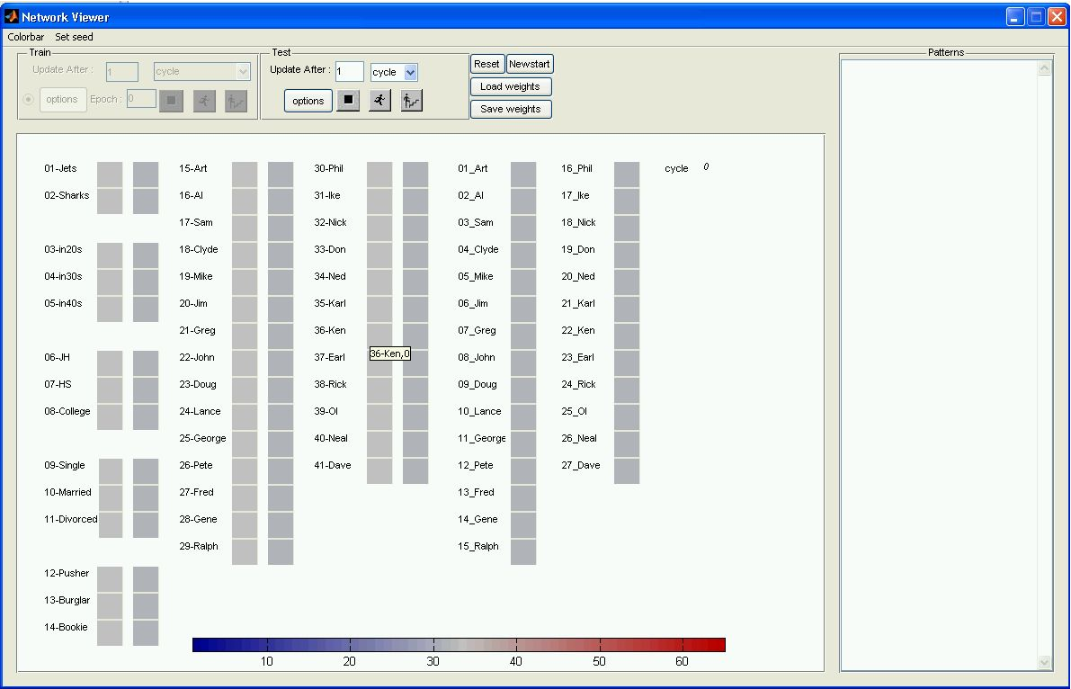
The program produces the display shown in Figure 2.3. The display shows the names of all of the units. Unit names are preceded by a two-digit unit number for convenience in some of the exercises below. The visible units are on the left in the display, and the hidden units are on the right. To the right of each visible unit name are two squares. The first square indicates the external input to the unit (which is initially 0). The second one indicates the activation of the unit, which is initially equal to the value of the rest parameter.

Since the hidden units do not receive external input, there is only one square to the right of the unit name for these units, for the unit’s activation. These units too have an initial activation activation level equal to rest.

On the far right of the display is the current cycle number, which is initialized to 0.

Since everything is set up for you, you are now ready to do each of the separate parts of the exercise. Each part is accomplished by using the interactive activation and competition process to do pattern completion, given some probe that is presented to the network. For example, to retrieve an individual’s properties from his name, you simply provide external input to his name unit, then allow the IAC network to propagate activation first to the name unit, then from there to the instance units, and from there to the units for the properties of the instance.

Retrieving an individual from his name. To illustrate retrieval of the properties of an individual from his name, we will use Ken as our example. Set the external input of Ken’s name unit to 1. Right-click on the square to right of the label 36-Ken. Type 1.00 and click enter. The square should turn red.

To run the network, you need to set the number of cycles you wish the network to run for (default is 10), and then click the button with the running man cartoon. The number of cycles passed is indicated in the top right corner of the network window. Click the run icon once now. Alternatively, you can click on the step icon 10 times, to get to the point where the network has run for 10 cycles.

The PDPtool programs offer a facility for creating graphs of units’ activations (or any other variables) as processing occurs. One such graph is set up for you. The panels on the left show the activations of units in each of the different visible pools excluding the name pool. The activations of the name units are shown in the middle. The activations of the instance units are shown in two panels on the right, one for the Jets and one for the Sharks. (If this window is in your way you can minimize (iconify) it, but you should not close it, since it must still exist for its contents to be reset properly when you reset the network.)

What you will see after running 10 cycles is as follows. In the Name panel, you will see one curve that starts at about .35 and rises rapidly to .8. This is the curve for the activation of unit 36-Ken. Most of the other curves are still at or near rest. (Explain to yourself why some have already gone below rest at this point.) A confusing fact about these graphs is that if lines fall on top of each other you only see the last one plotted, and at this point many of the lines do fall on top of each other. In the instance unit panels, you will see one curve that rises above the others, this one for hidden unit 22_Ken. Explain to yourself why this rises more slowly than the name unit for Ken, shown in the Name panel.

Two variables that you need to understand are the update after variable in the test panel and the ncycles variable in the testing options popup window. The former (update after) tells the program how frequently to update the display while running. The latter (ncycles) tells the program how many cycles to run when you hit run. So, if ncycles is 10 and update after is 1, the program will run 10 cycles when you click the little running man, and will update the display after each cycle. With the above in mind you can now understand what happens when you click the stepping icon. This is just like hitting run except that the program stops after each screen update, so you can see what has changed. To continue, hit the stepping icon again, or hit run and the program will run to the next stopping point (i.e. next number divisible by ncycles.

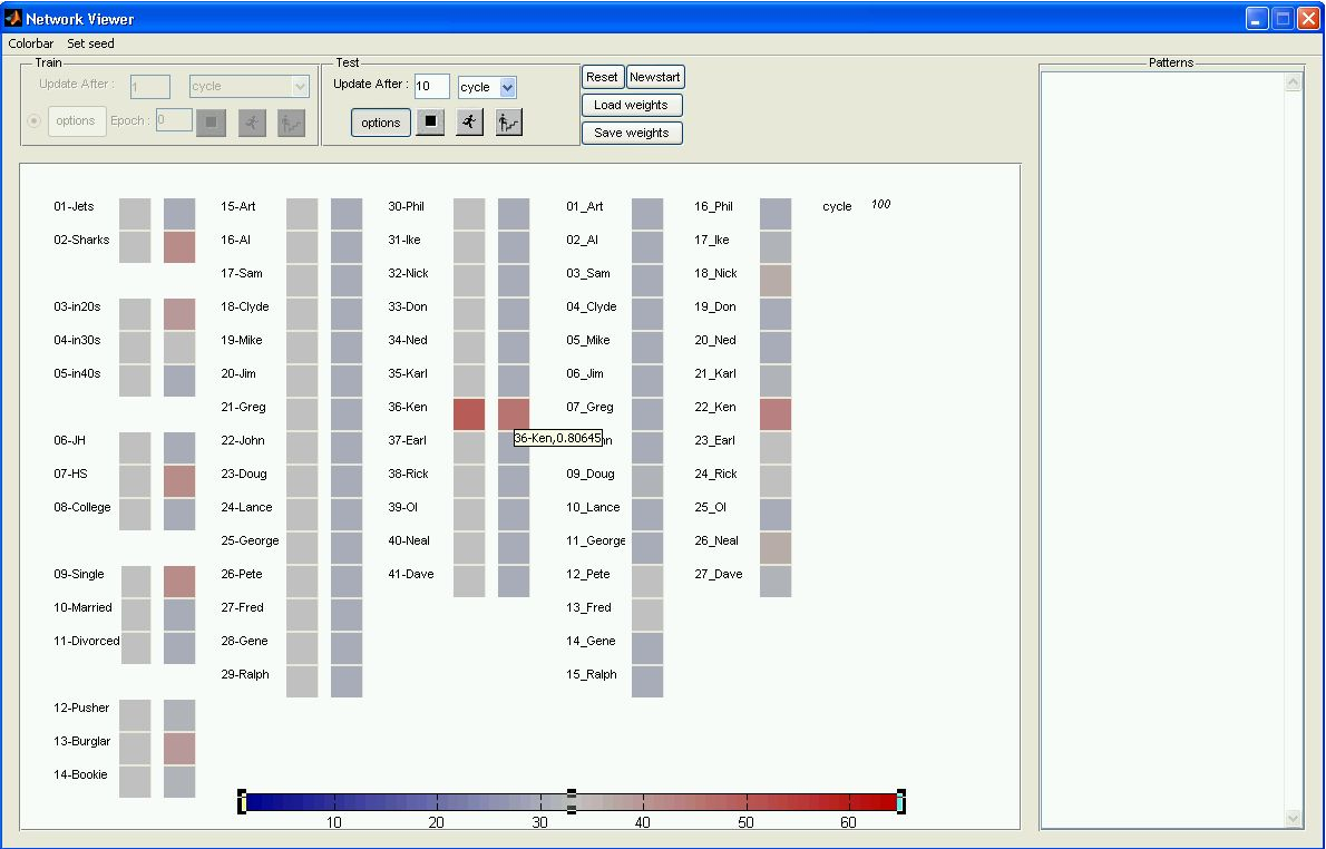
As you will observe, activations continue to change for many cycles of processing. Things slow down gradually, so that after a while not much seems to be happening on each trial. Eventually things just about stop changing. Once you’ve run 100 cycles, stop and consider these questions.

A picture of the screen after 100 cycles is shown in Figure 2.4. At this point, you can check to see that the model has indeed retrieved the pattern for Ken correctly. There are also several other things going on that are worth understanding. Try to answer all of the following questions (you’ll have to refer to the properties of the individuals, as given in Figure 2.1).

Q.2.1.1.

Q.2.1.2.

Save the activations of all the units for future reference by typing: saveVis = net.pool(2).activation and saveHid = net.pool(3).activation. Also, save the Figure in a file, through the ‘File’ menu in the upper left corner of the Figure panel. The contents of the figure will be reset when you reset the network, and it will be useful to have the saved Figure from the first run so you can compare it to the one you get after the next run.

Retrieval from a partial description. Next, we will use the iac program to illustrate how it can retrieve an instance from a partial description of its properties. We will continue to use Ken, who, as it happens, can be uniquely described by two properties, Shark and in20s. Click the reset button in the network window. Make sure all units have input of 0. (You will have to right-click on Ken and set that unit back to 0). Set the external input of the 02-Sharks unit and the 03-in20s unit to 1.00. Run a total of 100 cycles again, and take a look at the state of the network.

Q.2.1.3.

Q.2.1.4.

Default assignment. Sometimes we do not know something about an individual; for example, we may never have been exposed to the fact that Lance is a Burglar. Yet we are able to give plausible guesses about such missing information. The iac program can do this too. Click the reset button in the network window. Make sure all units have input of 0. Set the external input of 24-Lance to 1.00. Run for 100 cycles and see what happens. Reset the network and change the connection weight between 10_Lance and 13-Burglar to 0. To do that, type the following commands in the main MATLAB command prompt:

net.pool(3).proj(2).weight(10,13) = 0;

net.pool(2).proj(2).weight(13,10) = 0;

Run the network again for 100 cycles and observe what happens.

Q.2.1.5.

Spontaneous generalization. Now we consider the network’s ability to retrieve appropriate generalizations over sets of individuals—that is, its ability to answer questions like “What are Jets like?” or “What are people who are in their 20s and have only a junior high education like?” Click the ‘reset’ button in the network window. Make sure all units have input of 0. Be sure to reinstall the connections between 13-Burglar and 10_Lance (set them back to 1). You can exit and restart the network if you like, or you can use the up arrow key to retrieve the last two commands above and edit them, replacing 0 with 1, as in:

net.pool(3).proj(2).weight(10,13) = 1;

Set the external input of Jets to 1.00. Run the network for 100 cycles and observe what happens. Reset the network and set the external input of Jets back to 0.00. Now, set the input to in20s and JH to 1.00. Run the network again for 100 cycles; you can ask it to generalize about the people in their 20s with a junior high education by providing external input to the in20s and JH units.

Q.2.1.6.

Now that you have completed all of the exercises discussed above, write a short essay of about 250 words in response to the following question.

Q.2.1.7.

Ex2.2. Effects of Changes in Parameter Values

In this exercise, we will examine the effects of variations of the parameters estr, alpha, gamma, and decay on the behavior of the iac program.

Increasing and decreasing the values of the strength parameters. Explore the effects of adjusting all of these parameters proportionally, using the partial description of Ken as probe (that is, providing external input to Shark and in20s). Click the reset button in the network window. Make sure all units have input of 0. To increase or decrease the network parameters, click on the options button in the network window. This will open a panel with fields for all parameters and their current values. Enter the new value(s) and click ‘ok’. To see the effect of changing the parameters, set the external input of in20s and Sharks to 1.00. For each test, run the network til it seems to asymtote, usually around 300 cycles. You can use the graphs to judge this.

Q.2.2.1.

Relative strength of excitation and inhibition. Return all the parameters to their original values, then explore the effects of varying the value of gamma above and below 0.1, again providing external input to the Sharks and in20s units. Also examine the effects on the completion of Lance’s properties from external input to his name, with and without the connections between the instance unit for Lance and the property unit for Burglar.

Q.2.2.2.

Ex2.3. Grossberg Variations

Explore the effects of using Grossberg’s update rule rather than the default rule used in the IAC model. Click the ‘reset’ button in the network window. Make sure all units have input of 0. Return all parameters to their original values. If you don’t remember them, you can always exit and reload the network from the main pdp window. Click on the options button in the network window and change actfunction from st (Standard) to gr (Grossbergs rule). Click ‘ok’. Now redo one or two of the simulations from Ex. 2.1.

Q.2.3.1.

Hint.

Ex2.4. Construct Your Own IAC Network

Construct a task that you would find interesting to explore in an IAC network, along with a knowledge base, and explore how well the network does in performing your task. To set up your network, you will need to construct a .net and a .tem file, and you must set the values of the connection weights between the units. Appendix B and The PDPTool User Guide provide information on how to do this. You may wish to refer to the jets.m, jets.net, and jets.tem files for examples.

Q.2.4.1.

Hint.