In the previous chapter we showed how PDP networks could be used for content-addressable memory retrieval, for prototype generation, for plausibly making default assignments for missing variables, and for spontaneously generalizing to novel inputs. In fact, these characteristics are reflections of a far more general process that many PDP models are capable of -namely, finding near-optimal solutions to problems with a large set of simultaneous constraints. This chapter introduces this constraint satisfaction process more generally and discusses two models for solving such problems. The specific models are the schema model, described in PDP:14 and the Boltzmann machine, described in PDP:7. These models are embodied in the cs (constraint satisfaction) program. We begin with a general discussion of constraint satisfaction and some general results. We then turn to the schema model. We describe the general characteristics of the schema model, show how it can be accessed from cs, and offer a number of examples of it in operation. This is followed in turn by a discussion of the Boltzmann machine model.
Consider a problem whose solution involves the simultaneous satisfaction of a very large number of constraints. To make the problem more difficult, suppose that there may be no perfect solution in which all of the constraints are completely satisfied. In such a case, the solution would involve the satisfaction of as many constraints as possible. Finally, imagine that some constraints may be more important than others. In particular, suppose that each constraint has an importance value associated with it and that the solution to the problem involves the simultaneous satisfaction of as many of the most important of these constraints as possible. In general, this is a very difficult problem. It is what Minsky and Papert (1969) have called the best match problem. It is a problem that is central to much of cognitive science. It also happens to be one of the kinds of problems that PDP systems solve in a very natural way. Many of the chapters in the two PDP volumes pointed to the importance of this problem and to the kinds of solutions offered by PDP systems.
To our knowledge, Hinton was the first to sketch the basic idea for using parallel networks to solve constraint satisfaction problems (Hinton, 1977). Basically, such problems are translated into the language of PDP by assuming that each unit represents a hypothesis and each connection a constraint among hypotheses. Thus, for example, if whenever hypothesis A is true, hypothesis B is usually true, we would have a positive connection from unit A to unit B. If, on the other hand, hypothesis A provides evidence against hypothesis B, we would have a negative connection from unit A to unit B. PDP constraint networks are designed to deal with weak constraints (Blake, 1983), that is, with situations in which constraints constitute a set of desiderata that ought to be satisfied rather than a set of hard constraints that must be satisfied. The goal is to find a solution in which as many of the most important constraints are satisfied as possible. The importance of the constraint is reflected by the strength of the connection representing that constraint. If the constraint is very important, the weights are large. Less important constraints involve smaller weights. In addition, units may receive external input. We can think of the external input as providing direct evidence for certain hypotheses. Sometimes we say the input ”clamps” a unit. This means that, in the solution, this particular unit must be on if the input is positive or must be off if the input is negative. Other times the input is not clamped but is graded. In this case, the input behaves as simply another weak constraint. Finally, different hypotheses may have different a priori probabilities. An appropriate solution to a constraint satisfaction problem must be able to reflect such prior information as well. This is done in PDP systems by assuming that each unit has a bias, which influences how likely the unit is to be on in the absence of other evidence. If a particular unit has a positive bias, then it is better to have the unit on; if it has a negative bias, there is a preference for it to be turned off.
We can now cast the constraint satisfaction problem described above in the following way. Let goodness of fit be the degree to which the desired constraints are satisfied. Thus, goodness of fit (or more simply goodness) depends on three things. First, it depends on the extent to which each unit satisfies the constraints imposed upon it by other units. Thus, if a connection between two units is positive, we say that the constraint is satisfied to the degree that both units are turned on. If the connection is negative, we can say that the constraint is violated to the degree that the units are turned on. A simple way of expressing this is to let the product of the activation of two units times the weight connecting them be the degree to which the constraint is satisfied. That is, for units i and j we let the product wijaiaj represent the degree to which the pairwise constraint between those two hypotheses is satisfied. Note that for positive weights the more the two units are on, the better the constraint is satisfied; whereas for negative weights the more the two units are on, the less the constraint is satisfied. Second, the satistfaction of the constraint associated with the a priori strength or probability of the hypothesis is captured by including the activation of each unit times its bias, aibiasi, in the goodness measure. Finally, the goodness of fit for a hypothesis when direct evidence is available includes also the product of the input value times the activation value of the unit, aiinputi. The bigger this product, the better the system is satisfying this external constraint.
Having identified the three types of constraint, and having defined mathematically the degree to which each is satisfied by the state of a network, we can now provide an expression for the total goodness, or degree of constraint satisfaction, associated with the state. This overall goodness is the function we want the network to maximize as processing takes place. This overall goodness is just the sum over all of the weights of the constraint satisfaction value for each weight, plus the sum over all external inputs and biases of the constraint satisfaction associated with each one of them:
|
| (3.1) |
Note: In constraint satisfaction systems, we imagine there is only a single (bidirectional) weight between each pair of units; wij is really the same weight as wji. Thus, the double summation over weights in Equation 3.1 is deliberately constructed so that each unique weight is counted only once.
We have solved a particular constraint satisfaction problem when we have found a set of activation values that maximizes the function shown in the above equation. It should be noted that since we want to have the activation values of the units represent the degree to which a particular hypothesis is satisfied, we want our activation values to range between a minimum and maximum value, in which the maximum value is understood to mean that the hypothesis should be accepted and the minimum value means that it should be rejected. Intermediate values correspond to intermediate states of certainty. We have now reduced the constraint satisfaction problem to the problem of maximizing the goodness function given above. There are many methods of finding the maxima of functions. Importantly, John Hopfield (1982) noted that there is a method that is naturally and simply implemented in a class of PDP networks with symmetric wegiths. Under these conditions it is easy to see how a PDP network naturally sets activation values so as to maximize the goodness function stated above. To see this, first notice that the set of terms in the goodness function that include the activation of a given unit i correspond to the product of its current net input times its activation value. We will call this set of terms Gi, and write
 | (3.2) |
where, as usual for PDP networks, neti is defined as
 | (3.3) |
Thus, the net input to a unit provides the unit with information as to its contribution to the goodness of the entire network state. Consider any particular unit in the network. That unit can always behave so as to increase its contribution to the overall goodness of fit if, whenever its net input is positive, the unit moves its activation toward its maximum activation value, and whenever its net input is negative, it moves its activation toward its minimum value. Moreover, since the global goodness of fit is simply the sum of the individual goodnesses, a whole network of units behaving in such a way will always increase the global goodness measure. This can be demonstated more formally by examining the partial derivative of the overall goodness with respect to the state of unit i. If we take this derivative, all terms in which ai is not a factor drop out, and we are simply left with the net input:
 | (3.4) |
By definition, the partial derivative expresses how a change in ai will affect G. Thus, again we see that when the net input is positive, increasing ai will increase goodness, and when the net input is negative, decreasing ai will increase goodness.
It might be noted that there is a slight problem here. Consider the case in which two units are simultaneously evaluating their net inputs. Suppose that both units are off and that there is a large negative weight between them; suppose further that each unit has a small positive net input. In this case, both units may turn on, but since they are connected by a negative connection, as soon as they are both on the overall goodness may decline. In this case, the next time these units get a chance to update they will both go off and this cycle can continue. There are basically two solutions to this. The standard solution is not to allow more than one unit to update at a time. In this case, one or the other of the units will come on and prevent the other from coming on. This is the case of so-called asynchronous update. The other solution is to use a synchronous update rule but to have units increase their activation values very slowly so they can” feel” each other coming on and achieve an appropriate balance.
In practice, goodness values generally do not increase indefinitely. Since units can reach maximal or minimal values of activation, they cannot continue to increase their activation values after some point so they cannot continue to increase the overall goodness of the state. Rather, they increase it until they reach their own maximum or minimum activation values. Thereafter, each unit behaves so as to never decrease the overall goodness. In this way, the global goodness measure continues to increase until all units achieve their maximally extreme value or until their net input becomes exactly O. When this is achieved, the system will stop changing and will have found a maximum in the goodness function and therefore a solution to our constraint satisfaction problem.
When it reaches this peak in the goodness function, the goodness can no longer change and the network is said to have reached a stable state; we say it has settled or relaxed to a solution. Importantly, this solution state can be guaranteed only to be a local rather than a global maximum in the goodness function. That is, this is a hill-climbing procedure that simply ensures that the system will find a peak in the goodness function, not that it will find the highest peak. The problem of local maxima is difficult for many systems. We address it at length in a later section. Suffice it to say, that different PDP systems differ in the difficulty they have with this problem.
The development thus far applies to both of the models under discussion in this chapter. It can also be noted that if the weight matrix in an lAC network is symmetric, it too is an example of a constraint satisfaction system. Clearly, there is a close relation between constraint satisfaction systems and content-addressable memories. We turn, at this point, to a discussion of the specific models and some examples with each. We begin with the schema model of PDP:14.
The schema model is one of the simplest of the constraint satisfaction models, but, nevertheless, it offers useful insights into the operation of all of the constraint satisfaction models. Update in the schema model is asynchronous. That is, units are chosen to be updated sequentially in random order. When chosen, the net input to the unit is computed and the activation of the unit is modified. Once a unit has been chosen for updating, the activation process in the schema model is continuous and deterministic. The connection matrix is symmetric and the units may not connect to themselves (wii = 0).
The logic of the hill-climbing method implies that whenever the net input (neti) is positive we must increase the activation value of the unit, and when it is negative we must decrease the activation value. To keep activations bounded between 1 and 0, we use the following simple update rule:
if neti > 0
otherwise,

Note that in this second case, since neti is negative and ai is positive, we are decreasing the activation of the unit. This rule has two virtues: it conforms to the requirements of our goodness function and it naturally constrains the activations between 0 and 1. As usual in these models, the net input comes from three sources: a unit’s neighbors, its bias, and its external inputs. These sources are added. Thus, we have
 | (3.5) |
Here the constants istr and estr are parameters that allow the relative contributions of the input from external sources and that from internal sources to be readily manipulated.
The cs program implementing the schema model is much like iac in structure. It differs in that it does asynchronous updates using a slightly different activation rule, as specified above. cs consists of essentially two routines: (a) an update routine called rupdate (for random update), which selects units at random and computes their net inputs and then their new activation values, and (b) a control routine, cycle, which calls rupdate in a loop for the specified number of cycles. Thus, in its simplest form, cycle is as follows:
Thus, each time cycle is called, the system calls rupdate ncycles times, and updates the current cycle number (a second call to cycle will continue cycling where the first one left off). Note that the actual code includes checks to see if the display should be updated and/or if the process should be interrupted. We have suppressed those aspects here to focus on the key ideas.
The rupdate routine itself does all of the work. It randomly selects a unit, computes its net input, and assigns the new activation value to the unit. It does this nupdates times. Typically, nupdates is set equal to nunits, so a single call to rupdate, on average, updates each unit once:
The code shown here not only suppresses the checks for interupts and display updates; it also suppresses the fact that units are organized into pools and projections. Instead it represents in simple form the processing that would occur in a network with a single pool of units and a single matrix of connections. It is a constraint of the model, not enforced in the code, that the weight matrix must be symmetric and its diagonal elements should all be 0.
The basic structure of cs and the mechanics of interacting with it are identical to those of iac. The cs program requires a .net file specifying the particular network under consideration, and may use a .wts file to specify particular values for the weights, and a template (.tem) file that specifies what is displayed on the screen. It also allows for a .pat file for specifying a set of patterns that can be presented to the network. Once you are in MATLAB the cs the program can be accessed by entering ’pdp’ at the matlab command prompt, or by entering the name of the pre-defined example network that has been created.
The normal sequence for running the model may involve applying external inputs to some of the units, then clicking the run button to cause the network to cycle. The system will cycle ncycles times and then stop. The value of the goodness as well as the states of activations of units can be displayed every 1 or more update or every one or more cycle, as specified in the test control panel. The step command can be used to run the network just until the next mandated display update. Once cycling stops, one can step again, or continue cycling for another ncycles if desired. While cycling, the system can be interrupted with the stop button.
There are two ways to reinitialize the state of the network. One of these commands, newstart, causes the program to generate a new random seed, then re-seed its random number generator, so that it will follow a new random sequence of updates. The other command, reset, seeds the random number generator with the same random seed that was just used, so that it will go through the very same random sequence of updates that it followed after the previous newstart or reset. The user can also specify a particular value for the random seed to use after the next reset. This can be entered by clicking set seed in the upper left corner of the network viewer window. In this case, when reset is next called, this value of the seed will be used, producing results identical to those produced on other runs begun with this same seed.
The following options and parameters of the model may be specified via the options button under the Test window on the network viewer or the Set Testing options item under the Network menu in the main pdp window. They can also be set using the command settestopts(’param’,value) where param is the name of the parameter.
We offer two exercises using the cs program. We begin with an exercise on the schema model. In Ex. 3.1, we give you the chance to explore the basic properties of this constraint satisfaction system, using the Necker cube example in PDP:14 (originally from Feldman (1981)). The second exercise is introduced after a discussion of the problem of local maxima and of the relationship between a network’s probability of being in a state and that state’s goodness. In the second exercise, Ex. 3.2, we will explore these issues in a type of constraint satisfaction model called the Boltzmann machine.
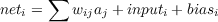
Feldman (1981) has provided a clear example of a constraint satisfaction problem well-suited to a PDP implementation. That is, he has shown how a simple constraint satisfaction model can capture the fact that there are exactly two good interpretations of a Necker cube. In PDP:14 (pp. 8-17), we describe a variant of the Feldman example relevant to this exercise. In this example we assume that we have a 16-unit network (as illustrated in Figure 3.1). Each unit in the network represents a hypothesis about the correct interpretation of a vertex of a Necker cube. For example, the unit in the lower left-hand part of the network represents the hypothesis that the lower left-hand vertex of the drawing is a front-lower-left (FLL) vertex. The upper right-hand unit of the network represents the hypothesis that the upper right-hand vertex of the Necker cube represents a front-upper-right (FUR) vertex. Note that these two interpretations are inconsistent in that we do not normally see both of those vertices as being in the frontal plane. The Necker cube has eight vertices, each of which has two possible interpretations-one corresponding to each of the two interpretations of the cube. Thus, we have a total of 16 units.
Three kinds of constraints are represented in the network. First, units that represent consistent interpretations of neighboring vertices should be mutually exciting. These constraints are all represented by positive connections with a weight of 1. Second, since each vertex can have only one interpretation, we have a negative connection between units representing alternative interpretations of the same input vertex. Also, since two different vertexes in the input can’t both be the same corner in the percept (e.g. there cannot be two front-lower-left corners when a single cube is perceived) the units representing the same corner of the cube in each of the interpretations are mutually inhibitory. These inhibitory connections all have weights of -1.5. Finally, we assume that the system is, essentially, viewing the ambiguous figure, so that each vertex gets some bottom up excitation. This is actually implemented through a positive bias equal to .5, coming to each unit in the network. The above values are all scaled by the istr parameter, which is set initially at .4 for this network.
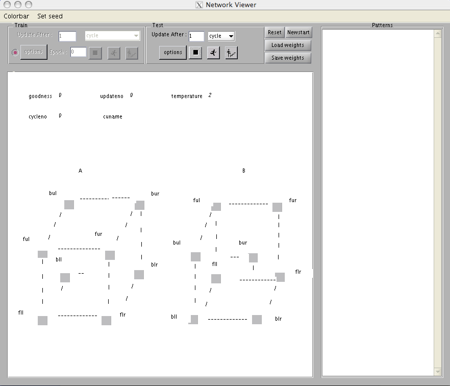
After setting the cs directory and the current directory, you can start up the cs program on the cube example by simply typing cube at the command prompt. At this point the screen should look like the one shown in Figure 3.2. The display depicts the two interpretations of the cube and shows the activation values of the units, the current cycle number, the current update number, the name of the most recently updated unit (there is none yet so this is blank), the current value of goodness, and the current temperature. (The temperature is irrelevant for this exercise, but will become important later.) The activation values of all 16 units are shown, initialized to 0, at the corners of the two cubes drawn on the screen. The units in the cube on the left, cube A, are the ones consistent with the interpretation that the cube is facing down and to the left. Those in the cube on the right, cube B, are the ones consistent with the interpretation of the cube as facing up and to the right. The dashed lines do not correspond to the connections among the units, but simply indicate the interpretations of the units. The connections are those shown in the Necker cube network in Figure 1. The vertices are labeled, and the labels on the screen correspond to those in Figure 3.1. All units have names. Their names are given by a capital letter indicating which interpretation is involved (A or B), followed by the label appropriate to the associated vertex. Thus, the unit displayed at the lower left vertex of cube A is named Afll, the one directly above it is named Aful (for the front-upper-left vertex of cube A), and so on.
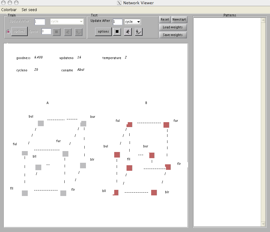
We are now ready to begin exploring the cube example. The biases and connections among the units have already been read into the program. In this example, as stated above, all units have positive biases, therefore there is no need to specify inputs. Simply click run. After the command is typed, the display will be updated once per cycle (that is, after every 16 unit updates). After the display stops flashing you should see the desplay shown in Figure 3.3. The variable cycle should be 20, indicating that the program has completed 20 cycles. The variable update should be at 16, indicating that we have completed the 16th update of the cycle. The uname will indicate the last unit updated. The goodness should have a value of 6.4. This value corresponds to a global maximum; and indeed, if you inspect the activations, you will see that the units on the right have reached the maximal value of one, and the units on the left are all 0, corresponding to one of the two “standard” interpretations of the cube.
Q.3.1.1.
Using 3.1, explain quantitatively how the exact value of goodness comes to be 6.4 when the network has reached the state shown in the display. Remember that all weights and biases are scaled by the istr parameter, which is set to .4. Thus each excitatory weight can be treated as having value .4, each inhibitory weight -.6, and the positive bias as having value .2.
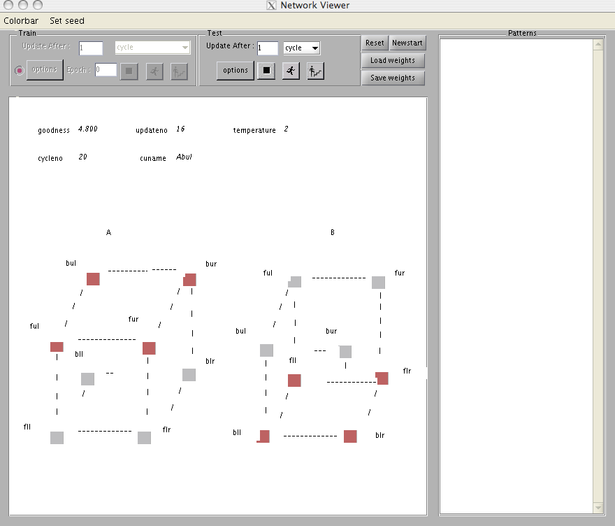
You can run the cube example again by issuing the newstart command and then hitting the run button. Do this until you find a case where, after 20 cycles, there are four units on in cube A and four on in cube B. The goodness will be 4.8.
Q.3.1.2.
Using 3.1, explain why the state you have found in this case corresponds to a goodness value of 4.8.
Continue again until you find a case where, after 20 cycles, there are two units on in one of the two cubes and six units on in the other.
Q.3.1.3.
Using Equation 3.1, explain why the state you have found in this case also corresponds to a goodness value of 4.8.
Now run about 20 more cases of newstart followed by run, and record for each the number of units on in each subnetwork after 20 cycles, making a simple tally of cases in which the result was [8 0] (all eight units in the left cube activated, none in the right), [6 2], [4 4], [2 6], and [0 8]. Examine the states where there are units on in both subnetworks.
To facilitate this process, we have provided a little function called onecube(n) that you can execute from the command line. This function issues one newstart and then runs n cycles, showing the final state only. To enter the command again, you can use ctrl-p, followed by enter. You can change the value of n by editing the command before you hit enter. For present purposes, you should simply leave n set at 20. Standalone users must follow the directions in this footnote.1
Q.3.1.4.
How many times was each of the two valid interpretations found? How many times did the system settle into a local maximum? What were the local maxima the system found? To what extent do they correspond to reasonable interpretations of the cube?
Now that you have a feeling for the range of final states that the system can reach, try to see if you can understand the course of processing leading up to the final state.
Q.3.1.5.
What causes the system to reach one interpretation or the other? How early in the processing cycle does the eventual interpretation become clear? What happens when the system reaches a local maximum? Is there a characteristic of the early stages of processing that leads the system to move toward a local maximum?
Hint.
Note that if you wish to study how the network evolved to a particular solution you obtained at the end of 20 cycles following a newstart, you can use reset to prepare the network to run through the very same sequence of unit updates again. If at that point you set Update after to 1 update, you can then then follow the steps to the solution update-by-update by clicking repeatedly on the step button. So, you can repeatedly issue the onecube(20) command until you find a case you’d like to study, click reset, set Update after as described, and step your way along to watch the state evolve.
There is a parameter in the schema model, istr, that multiplies the weights and biases and that, in effect, determines the rate of activation flow within the model. The probability of finding a local maximum depends on the value of this parameter. You can set this variable through the value of istr under the options popup under the test panel. Another way to set this is by using the command settestopts(’istr’,value) where value a positive number. Try several values from 0.1 to 2.0, running onecube 20 times for each.
Q.3.1.6.
How does the distribution of final states vary as the value of istr is varied? Report your results in table form for each value of istr, showing the number of times the network settles to [8 0], [6 2], [4 4], [2 6], and [0 8] in each case. Consider the distribution of different types of local maxima for different values of istr carefully. Do your best explain the results you obtain.
Hint.
At low values of istr you will want to increase the value of the ncycles argument to onecube; 80 works well for values like 0.1. Do not be disturbed by the fact that the values of goodness are different here than in the previous runs. Since istr effectively scales the weights and biases, it also multiplies the goodness so that goodness is proportional to istr.
Biasing the necker cube toward one of the two possible solutions. Although we do not provide an excise associated with this, we note that it is possible to use external inputs to bias the network in favor of one of the two interpretations. Study the effects of adding an input of 1.0 to some of the units in one of the subnetworks, using a command like the following at the command prompt:
The first eight units are for interpretation A, so this should provide external input (scaled by estr, which is set to the same .4 value as istr) to all eight of the units corresponding to that interpreation. If you wish, you can explore how the distribution of interpretations changes as a result of varying the number of units receiving external input of 1. You can also vary the strength of the external inputs, either by supplying values differet from 1 in the external input vector, or by adjusting the value of the estr parameter.
One other pre-defined network is available using the schema model. This is a network described in PDP:14 that is intended to illustrate various features of a PDP implementation of the idea of a ’schema’. Consult PDP:14 for a the background and for the details of this model.
The network is called the room network, and can be started (after closing other networks) by typing room to the Matlab command prompt while in the cs directory. The network can be used in either of two ways. The first involves setting external input values for one or a few of the units in the network, and then allowing the network to settle to a stable state (weights are symmetric so a fixed point will eventually be reached). To use the program in this way, simply provide external inputs by right clicking of the box to the left of the corresponding unit name, typing in a value, and hitting enter (the box to the right of the unit name represents the unit’s activation). These values are initialized to 0 at startup. You can actually run the program with no external inputs, and it will settle to a state that seems to be something like a bedroom, with a television and some bookshelves in it, and a fireplace. If you provide input to ’stove’, the network will settle to a very different state. You can play with different combinations, hitting reset then run after setting the desired extenal inputs. Remember to re-enter 0 values for external inputs you do not want to keep active.
The second way of using the room network involves clamping entire patterns corresponding to particular states onto the units. In this mode there is no real settling. Actiations are fixed to specific values (1 or 0) by the values specified in the patterns, which are contained in a file named ROOM.PAT. In this mode, while multiple cyles can occur, nothing happens to the activations because they are clamped, but the weights and activations are used to calculate goodness values for the specified states. These patterns are shown in the network view window after the program is launched. To use the program in this mode, click the Pat checkbox in the Test control panel. Click Reset to set activations back to 0 (although the display does not update after reset is clicked in this case). Then click on a pattern that you wish to present, then click the step icon in the Test control panel. You can explore other patterns most easily by adding your own patterns to the ROOM.PAT file or to a file of another name that you then load yourself – this file can be loaded through the Load new button within the testing options subpanel, then selecting your new file, which should be in the cs directory and have the .pat extension. Note that in the pattern file, a value of 1 is used to clamp a unit on and -1 is used to clamp the unit off.
In this section we introduce Hinton and Sejnowski’s Boltzmann machine, described in PDP:7. This model was developed from an analogy with statistical physics and it is useful to put it in this context. We thus begin with a description of the physical analogy and then show how this analogy solves some of the problems of the schema model described above. Then we turn to a description of the Boltzmann machine, show how it is implemented, and allow you to explore how the cs program can be used in boltzmann mode to address constraint satisfaction problems.
The initial focus of this material when first written in the 1980’s was on the use of the Boltzmann machine to solve the problem of local maxima. However, an alternative, and perhaps more important, perspective on the Boltzmann machine is that is also provides an important step toward a theory of the relationship between the content of neural networks (i.e. the knowledge in the weights) and the probability that they settle to particular outcomes. We have already taken a first step in the direction of such a theory, by seeing that networks tend to seek maxima in Goodness, which is in turn related to the knowledge in the weights. In this section we introduce an elegant analysis of the quantitative form of the relationship between the probability that a network will find itself in a particular state, and that state’s Goodness. Because of the link between goodness and constraints encoded in the weights this analysis allows a deeper understanding of the relationship between the constraints and the outcome of processing.
As stated above, one advantage of the Boltzmann machine over the deterministic constraint satisfaction system used in the schema model is its ability to overcome the problem of local maxima in the goodness function. To understand how this is done, it will be useful to begin with an example of a local maximum and try to understand in some detail why it occurs and what can be done about it. Figure 3.4 illustrates a typical example of a local maximum with the Necker cube. Here we see that the system has settled to a state in which the upper four vertices were organized according to interpretation A and the lower four vertices were organized according to interpretation B. Local maxima are always blends of parts of the two global maxima. We never see a final state in which the points are scattered randomly across the two interpretations.
All of the local maxima are cases in which one small cluster of adjacent vertices are organized in one way and the rest are organized in another. This is because the constraints are local. That is, a given vertex supports and receives support from its neighbors. The units in the cluster mutually support one another. Moreover, the two clusters are always arranged so that none of the inhibitory connections are active. Note in this case, Afur is on and the two units it inhibits, Bfur and Bbur, are both off. Similarly, Abur is on and Bbur and Bfur are both off. Clearly the system has found little coalitions of units that hang together and conflict minimally with the other coalitions. In Ex. 3.1, we had the opportunity to explore the process of settling into one of these local maxima. What happens is this. First a unit in one subnetwork comes on. Then a unit in the other subnetwork, which does not interact directly with the first, is updated, and, since it has a positive bias and at that time no conflicting inputs, it also comes on. Now the next unit to come on may be a unit that supports either of the two units already on or possibly another unit that doesn’t interact directly with either of the other two units. As more units come on, they will fit into one or another of these two emerging coalitions. Units that are directly inconsistent with active units will not come on or will come on weakly and then probably be turned off again. In short, local maxima occur when units that don’t interact directly set up coalitions in both of the subnetworks; by the time interaction does occur, it is too late, and the coalitions are set.
Interestingly, the coalitions that get set up in the Necker cube are analogous to the bonding of atoms in a crystalline structure. In a crystal the atoms interact in much the same way as the vertices of our cube. If a particular atom is oriented in a particular way, it will tend to influence the orientation of nearby atoms so that they fit together optimally. This happens over the entire crystal so that some atoms, in one part of the crystal, can form a structure in one orientation while atoms in another part of the crystal can form a structure in another orientation. The points where these opposing orientations meet constitute flaws in the crystal. It turns out that there is a strong mathematical similarity between our network models and these kinds of processes in physics. Indeed, the work of Hopfield (1982, 1984) on so-called Hopfield nets, of Hinton and Sejnowski (1983), PDP:7, on the Boltzmann machine, and of Smolensky (1983), PDP:6, on harmony theory were strongly inspired by just these kinds of processes. In physics, the analogs of the goodness maxima of the above discussion are energy minima. There is a tendency for all physical systems to evolve from highly energetic states to states of minimal energy. In 1982, Hopfield, (who is a physicist), observed that symmetric networks using deterministic update rules behave in such a way as to minimize an overall measure he called energy defined over the whole network. Hopfield’s energy measure was essentially the negative of our goodness measure. We use the term goodness because we think of our system as a system for maximizing the goodness of fit of the system to a set of constraints. Hopfield, however, thought in terms of energy, because his networks behaved very much as thermodynamical systems, which seek minimum energy states. In physics the stable minimum energy states are called attractor states. This analogy of networks falling into energy minima just as physical systems do has provided an important conceptual tool for analyzing parallel distributed processing mechanisms.
Hopfield’s original networks had a problem with local ”energy minima” that was much worse than in the schema model described earlier. His units were binary. (Hopfield (1984) subsequently proposed a version in which units take on a continuum of values to help deal with the problem of local minima in his original model. The schema model is similar to Hopfield’s 1984 model, and with small values of istr we have seen that it is less likely to settle to a local minimum). For binary units, if the net input to a unit is positive, the unit takes on its maximum value; if it is negative, the unit takes on its minimum value (otherwise, it doesn’t change value). Binary units are more prone to local minima because the units do not get an opportunity to communicate with one another before committing to one value or the other. In Ex. 3.1, we gave you the opportunity to run a version close to the binary Hopfield model by setting istr to 2.0 in the Necker cube example. In this case the units are always at either their maximum or minimum values. Under these conditions, the system reaches local goodness maxima (energy minima in Hopfield’s terminology) much more frequently.
Once the problem has been cast as an energy minimization problem and the analogy with crystals has been noted, the solution to the problem of local goodness maxima can be solved in essentially the same way that flaws are dealt with in crystal formation. One standard method involves annealing. Annealing is a process whereby a material is heated and then cooled very slowly. The idea is that as the material is heated, the bonds among the atoms weaken and the atoms are free to reorient relatively freely. They are in a state of high energy. As the material is cooled, the bonds begin to strengthen, and as the cooling continues, the bonds eventually become sufficiently strong that the material freezes. If we want to minimize the occurrence of flaws in the material, we must cool slowly enough so that the effects of one particular coalition of atoms has time to propagate from neighbor to neighbor throughout the whole material before the material freezes. The cooling must be especially slow as the freezing temperature is approached. During this period the bonds are quite strong so that the clusters will hold together, but they are not so strong that atoms in one cluster might not change state so as to line up with those in an adjacent cluster even if it means moving into a momentarily more energetic state. In this way annealing can move a material toward a global energy minimum.
The solution then is to add an annealing-like process to our network models and have them employ a kind of simulated annealing. The basic idea is to add a global parameter analogous to temperature in physical systems and therefore called temperature. This parameter should act in such a way as to decrease the strength of connections at the start and then change so as to strengthen them as the network is settling. Moreover, the system should exhibit some random behavior so that instead of always moving uphill in goodness space, when the temperature is high it will sometimes move downhill. This will allow the system to ”step down from” goodness peaks that are not very high and explore other parts of the goodness space to find the global peak. This is just what Hinton and Sejnowski have proposed in the Boltzmann machine, what Geman and Geman (1984) have proposed in the Gibbs sampler, and what Smolensky has proposed in harmony theory. The essential update rule employed in all of these models is probabilistic and is given by what we call the logistic function:
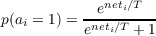 | (3.6) |
where T is the temperature. Dividing the numerator and denominator by eneti∕T gives the following version of this function, which is the one must typically used:
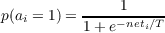 | (3.7) |
This differs from the basic schema model in several important ways. First, like Hopfield’s original model, the units are binary. They can only take on values of 0 and 1. Second, they are stochastic – that is, their value is subject to uncertainty. The update rule specifies only a probability that the units will take on one or the other of their values. This means that the system need not necessarily go uphill in goodness-it can move downhill as well. Third, the behavior of the systems depends on a global parameter, T, which determines the relative likelihood of different states in the network.
In fact, in networks of this type, a very important relationship holds betwen the equilibrium probability of a state and the state’s goodness:
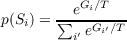 | (3.8) |
The denominator of this expression is a sum over all possible states, and is often difficult to compute, but we now can see the likehood ratio of being in either of two states S1 or S2 is given by
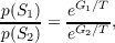 | (3.9) |
or alternatively,
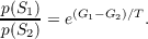 | (3.10) |
A final way of looking at this relationship that is sometimes useful comes if we take the log of both sides of this expression:
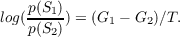 | (3.11) |
At equilibrium, the log odds of the two states is equal to the difference in goodness, divided by the temperature.
These simple expressions above can serve two important purposes for neural network theory. First, they allow us to predict what a network will do from knowledge of the constraints encoded in its weights, biases, and inputs, when the network is run at a fixed temperature. This allows a mathematical derivation of aspects a network’s behavior and it allows us to relate the network’s behavior to theories of optimal inference.
Second, these expressions allow us to prove that we can, in fact, find a way to have networks settle to one of their global maxima. In essence, the reason for this is that, as T grows small, the probility ratios of particular pairs of states become more and more extreme. Consider two states with Goodness 5 and goodness 4. When T is 1, the ratio of the probabilities is e, or 2.73:1. But when the temperature is .1, the ratio e10, or 22,026:1. In general, as temperature goes down we can make the ratio of the probabilities of two states as large as we like, even if the goodness difference between their probabilities is small.
However, there is one caveat. This is that the above is true, only at equilibrium, and provided that the system is ergodic.
The equilibrium probability of a state is a slightly tricky concept. It is best understood by thinking of a very large number of copies of the very same network, each evolving randomly over time (with a different random seed, so each one is different). Then we can ask: What fraction of these networks are in any given state at any given time? They might all start out in the same state, and they may all tend to evolve toward better states, but at some point the tendency to move into a good state is balanced by the tendency to move out of it again, and at this point we say that the probability distribution has reached equilibrium. At moderate temperatures, the flow between states occurs readily, and the networks tend to follow the equilibrium distribution at they jump around from state to state. At low temperatures, however, jumping between states becomes very unlikely, and so the networks may be more likely to be found in local maxima than in states that are actually better but are also neighbors of even better states. When the flow is possible, we say that the system is ergodic. When the system is ergotic, the equilibrium is independent of the starting state. When the flow is not completely open, it is not possible to get from some states to some other states.
In practice “ergodicity” is a matter of degree. If nearby relatively bad states have very low probability of being entered from nearly higher states, it can simply take more time that it seems practical to wait for much in the way of flow to occur. This is where simulated annealing comes in. We can start with the temperature high, allowing a lot of flow out of relatively good states and gradually lower the temperature to some desired level. At this temperature, the distribution of states can in some cases approximate the equilibrium distribution, even though there is not really much ongoing movement between different states.
To get a sense of all of this, we will run a few more exercises. Each exercise will involve running an ensemble of networks (100 of them) and then looking at the distribution across states at the end of some number of cycles. Luckily, we are using a simple network, so running an ensemble of them goes quickly.
To start this exercise, exit from the cube example through the pdp window (so that all your windows close). To make sure everything is cleared up, you can type
at the command prompt. Then start up again using the command boltzcube to the command prompt. What is different about this compared to cube is that the model is initiated in Boltzmann mode, with an annealing schedule specified, and both istr and estr are set to 1 so that the goodness values are more transparent. The two global optima are associated with goodness of 16. This consists of 12 times 1 for the weights along the edges of the interpretation in which all of the units are active, plus 8 times .5 for the bias inputs to the eight units representing the corners of that cube. The local maxima we have considered all have goodness of 12.
The annealing schedule can be set through the options popup (annealsched pushbutton) but is in fact easier to specify at the command prompt via the settestopts command. Throughout this exercise, we will work with a final temperature of 0.5. The initial annealing schedule is set in the script by the command:
This tells the network to initialize the temperature at 2, then linearly reduce it over 20 cycles to .5. In general the schedule consists of a set of time value pairs, separated by a semicolon. Times must increase, and values must be greater than 0 (use .001 if you want effectively 0 temperature).
Each time you run an ensemble of networks, you will do so using the manycubes command. This command takes two arguments. The first is the number of instances of the network settling process to run and the second is the number of cycles to use in running each instance. Enter the command shown below now at the command prompt with arguments 100 and 20, to run 100 instances of the network each for 20 cycles. Standalone users must follow the directions in this footnote.2
If you have the Network Viewer window up on your screen, you’ll see the initial and final states for each instance of the settling process flash by one by one. At the end of 100 instances, a bargraph will pop up, showing the distribution of goodness values of the states reached after 20 cycles. The actual numbers corresponding to the bars on the graph are stored in the histvals variable; there are 33 values corresponding to goodnesses from 0 to 16 in steps of 0.5. Enter histvals(17:33) to display the entries corresponding to goodness values from 8 to 16. In one run of the manycubes(100,20), the results came out like this:
We want to know whether we are getting about the right equilibrium distribution of states, given that our final temperature is .5. We can calculate the ratios of probabilities of being in particular states, but we need to take into account that in fact there are several states with each of the four goodness values mentioned above. The probability of having a particular goodness is equal to the probability of being in a particular state with that goodness times the number of such states.
Q.3.2.1.
How many different states of the network have goodness values of 16? Here, it is immediately obvious that there are two such states. How many local maxima are there, that have goodness values of 12? Consider, also, the state in which all but one unit is on in one cube and no units are on in the other. What is the goodness value of that state? How many such states are there? Finally, consider the states in which all units are on in one cube, and one is on in the other. What is the goodness value of such a state? How many such states are there? Although the answers are given below you should try to work this out yourself first, then, in your written answer, explain how you get these numbers.
Since we need to have the right numbers to proceed, we give the answers to the question above:
If your answer differs with regard to the number of goodness 12 states, here is an explanation. Competition occurs between pairs of units in the two cubes corresponding to the two alternative interpretations of each of the four front-to-back edges. Either pair of units can be on without direct mutual inhibitory conflict. Other edges of the cubes do not have this property. There are thus four ways to have an edge missing from one cube, and four ways to have an edge missing from the other cube. Thus there are four 6-2 and four 2-6 maxima. Similarly, the top surface of cube A can coexist with the bottom surface of cube B (or vise versa) without mutual inhibition, and the left surface of cube A can coexist with the right surface of cube B (or vice versa) without mutual inhibition, giving four possible 4-4 local maxima. Note that the four units corresponding to the front or back surface of cube A cannot coexist with the four units corresponding to either the front or the back surface of cube B due to the mutual inhibition.
So now we can finally ask, what is the relative probability of being in a state with one of these four goodnesses, given the final temperature achieved in the network?
We can calculate this as follows. For each Goodness Value (GV ), we have:
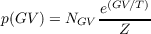 | (3.12) |
Here NGV represents the number of different states having the goodness value in question, and e(GV∕T) is proportional to the probability of being in any one of these states. We use Z to represent the denominator, which we will not need to calculate. Consider first the value of this expression for the highest goodness value, GV = 16, corresponding to the global maxima. There are two such maxima, so NGV = 2. So to calculate the numerator of this expression (disregarding Z) for our temperature T = .5, we enter the following at or MATLAB command prompt:
We see this is a very large number. To see it in somewhat more compact format enter format short g at the MATLAB prompt then enter the above expression again. The number is 1.58 times 10 to the 14th power. Things come back into perspective when we look at the ratio of the probability of being in a state with goodness 16 to the probability of being in a state with goodness 13.5. There are 16 such states, so the ratio is given by:
The ratio is manageable: it is 18.6 or so. Thus we should have a little more than 18 times as many states of goodness 16 as we have states of goodness 13.5. In fact we are quite far off from this in my run; we have 62 cases of states of goodness 16, and 14 cases of states of goodness 13.5, so the ratio is 4.4 and is too low.
Let’s now do the same thing for the ratio of states of goodness 12 to states of goodness 16. There are 12 states of goodness 12, so the ratio is entered as
Calculating, we find this ratio is 496.8. Since I observed 10 states of goodness 12, and 62 of goodness 16, the observed ratio is hugely off: 62∕10 is only 6.2.
Looking at the probability ratio for states of goodness 12.5 vs. 12, we have:
The ratio is 3.6. Thus, at equilibrium the network should be in a 12.5 goodness state more often than a 12 goodness state. However, we have the opposite pattern, with 10 instances of goodness 12 and 2 of goodness 12.5. Clearly, we have not achieved an approximation of the equilibrium distribution; it appears that many instances of the network are stuck in one of the local maxima, i.e. the states with goodness of 12.
The approximate expected counts of 100 samples at equilibrium should be:
| Goodness | Expected Count |
| 16 | 93.1 |
| 13.5 | 5.0 |
| 12.5 | 0.7 |
| 12 | 0.2 |
| All others | 1.0 |
Q.3.2.2.
Try to find an annealing schedule that runs over 100 cycles with a final temperature of 0.5 that ends up as close as possible to the right final distribution over the states with goodness values of 16, 13.5, 12.5, and 12. (Some lower goodness values may also appear.) In particular, try to find a schedule that produces 1 or fewer states with a goodness value of 12. You’ll need to do several runs of 100 cycles, 100 instances each using the manycubes command. Report the results of your best annealing schedule and three other schedules in a table, showing the annealing schedules used as well as the number of states per goodness value (between 8 and 16) at the end of each run. For your best schedule, report the results of two runs, since there is variability from run to run. Explain the adjustments you make to the annealing schedule and the thoughts that led you to make them.
To make your life easy you can use a command like
with no semi-colon at the end to show the entries in histvals corresponding to goodnesses ranging from 8 (histvals(17)) to 16 (histvals(33)). The bargraph will make it easy to get a sense is what is going on while the screen dump of the numbers gives you the actual values.
If the line before the call to manycubes sets the annealing schedule (see example below), then the main MATLAB window will contain a record of all of your commands and all of your data, and you can copy and paste individual lines into your homework paper; of course, you will want to edit and reformat for readability. Remember you can use the arrow keys to access previous commands and that you can edit them before hitting enter.
In adjusting the annealing schedule, you will want to consider whether the intial temperature is high enough. Thus, if you want to use a higher start value and an intermediate milestone, you might have the following commands (note that the total number of cycles is specified in both the annealing schedule and manycubes commands):
Hint.
A higher initial temperature with two intermediate milestones produces results that come close to matching the correct equilibrium distribution. It is hard to get a perfect match – see what you come up with.
The next question harkens back to the discussion of the physical process of annealing in the discussion of the physics analogy:
Q.3.2.3.
Discuss the likelihood of a network escaping from a [4 4] local maximum to another local maximum at T = 1: Provide an example of 2 sequences of evens by which this might occur. Picking one such sequence, calculate the probability that such a series of states would occur. Once such a maximum is escaped to a global maximum, what sequence of events would have to happen to get back to this [4 4] local maximum? Also consider excape and return to [6 2] and [2 6] type local maxima. We don’t expect exact answers here, but the question will hopefully elicit reasonable intuitions. With these thoughts in hand, discuss your understanding of why your best schedule reported above works as well or poorly as it does, and how you might improve on it further.
The title of this section is a bit of a play on words. We have been focusing on local maxima, and how to escape from them, in a way that may distract from the deeper contribution of the relationship between goodness and probability. For example, it may be that local maxima are not as much of a problem in PDP systems as the cube example makes it seem like they might be. The constraints used in this example were deliberately chosen to create a network that would have such maxima, so that it would help illustrate several useful concepts. But are local maxima inevitable?
Q.3.2.4.
Consider how you might change the network used in the cube example to avoid the problem of local maxima. Assume you still have the same sixteen vertex units, and the same bias inputs making each of the two interpretations equally likely. Briefly explain (with an optional drawing) one example in which adding connections would help and one example in which adding hidden units would help.
Your answer may help to illustrate both that local maxima are not necessarily inevitable and that hidden units (units representing important clusters of inputs that tend to occur together in experience) may play a role in solving the local maximum problem. More generally, the point here is to suggest that the relationship between constraints, goodness, and probability may be a useful one even beyond avoiding the problem of getting stuck in local maxima.