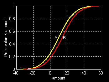
An Investor must choose between two portfolios. The end-of-period value of each one is normally distributed. Portfolio A has an expected value of $10,000 and a standard deviation of $15,000. Portfolio B has an expected return of $14,000 and a standard deviation of $15,000. Which will provide the greatest expected utility?
The answer is not difficult to obtain. As long as the Investor's utility increases with wealth and does not depend on the state of the world in which the wealth is obtained, portfolio B is better. This can be seen in the plot of the cumulative distributions, shown below:

Take any possible outcome -- for example, $5,000. This is (5,000-10,000)/15,000 standard deviations from the expected value of portfolio A. The probability that the actual outcome will fall short of this amount is cnd((5000-10000)/15000) or 0.3694. On the other hand, this outcome is (5,000-14,000)/15,000 standard deviations from the expected value of portfolio B. The probability that the actual outcome will fall short of this amount is cnd((5000-14000)/15000) or 0.2743. Clearly, it is better to have a smaller chance of a shortfall below $5,000; in this respect, B is preferred to A. But the result will be the same for every possible outcome, as the figure shows. Portfolio B thus dominates portfolio A for any Investor who prefers more wealth to less and who has a state-independent utility function. Formally, this is termed a case of first-degree stochastic dominance. More simply put: mean-variance theory assumes that among portfolios with the same standard deviation, the one with the greatest expected value is the best.
Now examine the figure below in which each circle plots the expected value and standard deviation of a different portfolio.
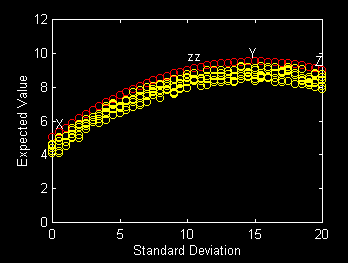
Consider the portfolios shown by the red circles in the figure that plot on curve XzzYZ. Each provides the maximum expected value for a given level of standard deviation. If all the portfolio returns are normally distributed, then any Investor for whom more wealth is better than less and for whom only wealth matters should choose from among the portfolios on this curve.
What about the portfolios on the section of the curve from Y to Z? The one plotting at point Y provides a greater expected value and a smaller standard deviation than any of the portfolios between Y and Z. Moreover, for every portfolio on the section between Y and Z there are alternatives with the same expected return but lower standard deviations. For example, portfolio zz offers the same expected return as Z but a lower standard deviation (indeed, the lowest possible, in this case). The figure below plots the cumulative distributions for these two portfolios.
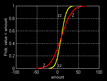
Portfolio zz dominates Z over the lower half of the range of possible outcomes, but Z provides larger chances of obtaining higher values.
To deal with such a case, Markowitz proposed that Investors be assumed to be risk-averse -- more precisely, each Investor's marginal utility of wealth is assumed to decline with wealth.
In this case, an Investor with decreasing marginal utility of wealth will prefer zz to Z, since moving from Z to zz will improve bad outcomes symmetrically with reductions in good outcomes, and the gain in utility from each of the former reductions will exceed the loss in utility from the corresponding latter reduction. Formally, this is a case of second-degree stochastic dominance.
Mean-variance theory assumes that Investors prefer (1) higher expected returns for a given level of standard deviation and (2) lower standard deviations for a given a level of expected return. Portfolios that provide the maximum expected return for a given standard deviation and the minimum standard deviation for a given expected return are termed efficient portfolios. All others are inefficient.
In practice the curve plotting the maximum expected value for each level of risk will usually be upward-sloping throughout the range of feasible values. Sections such as YZ are rare. Thus it generally suffices to assume only that Investors prefer greater expected return for given risk, placing a considerably smaller burden on the Analyst who advocates a focus on only efficient portfolios.
The figure below provides an illustration, with expected returns expressed in terms of excess returns over and above a riskless rate of interest.
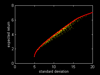
In this figure each point represents a portfolio. Given the Investor's budget and the joint distribution of security and portfolio values, there are many such points, only a few of which are shown in the figure. The set of all such points make up a feasible region of mean-variance (or mean-standard deviation) combinations. Efficient portfolios plot on the upper left-hand border of this region, shown as a red curved line in this case. For obvious reasons this border is often termed the efficient frontier.
By its nature, our delineation of the roles of the Analyst and the Investor suggests a division of labor. The Analyst is presumed to be an expert on capital markets, while the Investor knows his or her circumstances, tastes, obligations, future opportunities, etc.. Their joint goal is to bring all this information together to achieve the best possible plan for the Investor's savings and investment.
Central in this enterprise is the selection of an asset mix for a long-term investment policy. Such a policy asset mix plays a key role in many investment plans. Its choice is often the first (and sometimes the only) joint undertaking of the Analyst and the Investor.
In principle, four ingredients are needed for a complete analysis of this type. In discrete terms: (1) estimates of possible payments made by various investment products at different times and in different states of the world, (2) estimates of the probabilities associated with these times and states of the world, (3) the Investor's utility function for consumption at different times and in different states of the world, and (4) the Investor's current wealth, projected future income and required payments at various times in various states of the world. Since the first two aspects are the same for every Investor, it pays to share the cost of obtaining information about them among many Investors. Economies of scale thus provide the primary justification for the existence of the Analyst, to whom this material is directed.
In mean-variance analyses, payments (item 1) and probabilities (item 2) are summarized in the mean-variance feasible region. By assuming that all Investors are risk-averse, the Analyst can narrow the range of "sensible" investment opportunities to those that lie on the efficient frontier. In some cases this may suffice. The dialogue would be something like this:
     Analyst: Here is the tradeoff between risk (standard deviation)
     and (expected) return, using only efficient strategies.  Which
     point do you want?

     Investor: I'll take that one (chooses a point).

     Analyst: OK.  The asset mix for you is (writes down a mix, which
     indicates the percentage to be invested in each of several asset
     classes).
In practice it is rarely this simple. While the mean-variance framework deals with only one period, actual investment policies are designed to last for many periods. Few Investors can relate one-period mean and variance to long-run outcomes. In most cases it falls to the Analyst to do so, taking into account information supplied by the Investor -- information that is unique to his or her situation.
Take the example of a 55-year old with savings of $500,000. She plans to save an additional $50,000 per year for the next ten years, then "cash in" and move to Southern France. She cares only about the amount of money that she will have at that time.
In such a circumstance an Analyst would generally do an asset allocation study. For example, five asset mixes might be selected from the efficient frontier, in order of increasing risk and expected return. For each mix a Monte Carlo analysis would be performed to estimate the probability distribution of the size of the Investor's retirement fund ten years hence. These would be shown to the Investor, who would pick the one she preferred. The dialogue would be something like:
     Analyst:  Based on your current and planned future savings, I
     have estimated the likely range of retirement funds for each of
     five efficient investment strategies.  The more conservative
     strategies run less risk of a truly disappointing outcome, but
     are likely to provide less under expected conditions.  Here are
     depictions that show what might happen with each policy.  Which
     do you prefer?

     Investor:  This is not an easy choice.  All things considered,
     this one (chooses a policy) seems best for me.

     Analyst: OK, here's the asset mix for you ....
Mean-variance theory provides a neat separation between Investor preferences and capital market opportunities. The latter are summarized in the feasible mean-variance opportunity set and its efficient frontier. The former can be shown with a set of Investor indifference curves
The diagram below shows portions of a map of the preferences of a specific Investor
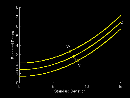
Here are some answers obtained when this Investor was asked to choose between various pairs of mean-variance combinations:
   Choose between     Answer
   --------------   -----------
      W and Y           W
      V and Y           Y
      X and Y        don't care
      W and Z           W
      V and X           X
      Z and Y        don't care
These responses can be written using algebraic notation, with > meaning "is preferred to" (more properly: "would be chosen over"), < the converse, and = meaning "is equally desirable as" (more properly, "would let someone else choose" or "flip a coin"). Thus:
      W > Y
      Y > V
      X = Y
      W > Z
      X > V
      Z = Y
If the Investor has transitive preferences, we can combine all these responses, using the rules of algebra:
W > X = Y = Z > V
Thus if we know that W is preferred to Y and Y is preferred to V, we assume that if asked to choose between W and V, the Investor would pick W. This may seem obvious, but people often fail to make choices that are "rational" in this sense. Worse yet, when the preferences represent the results of choices made by a committee voting by majority rule, instances of intransitivity are common. In such cases the order in which votes are presented can easily affect the outcome. Thus W might win over Y in a first vote, and Y over V in a second vote, even though in an initial contest between W and V, the victory might have gone to V.
The Analyst who works with Investment Committees must be aware of such possibilities: a difficult task indeed. Such is the world of practice. In the world of theory no such dangers lurk. The Investor is assumed to have transitive preferences which can, in principle, be graphed as a series of indifference curves of the type shown in the figure. The Investor is indifferent among all combinations of expected return and risk plotting on a single indifference curve (for example, X,Y and Z). He or she prefers any combination on a curve that cuts the expected return axis at a higher point to any combination that cuts it at a lower point. Thus W is preferred to X (or Y or Z or V), and X (or Y or Z) is preferred to V. The joint task of the Investor and the Analyst is to put the former on the highest possible indifference curve. This is shown below, with the red curve plotting the risk and return combinations available with efficient portfolios.
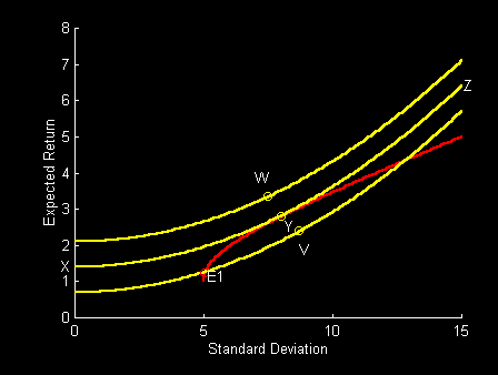
In this case, point Y is optimal. Note that point E1 is inferior. Even though it represents an efficient mean-variance combination, it puts the Investor on the lowest curve shown, points on which are inferior to points on the middle curve, given his or her preferences. Of course, this Investor would prefer to be on the highest curve shown, but this is impossible, given current resources and capital market opportunities.
It would be convenient if each Investor would present an Analyst with a complete map of his or her indifference curves. The Analyst could then recommend an asset mix virtually instantaneously. But the task is never this simple. As we will see, indifference curves are a useful construct, but in practice the Analyst generally focuses on only one portion of an Investor's entire indifference map -- which is just as well
Mean-variance theory assumes that every Investor's utility function increases at a decreasing rate as wealth increases and is independent of the state of the world in which wealth is received. Even for Investors for whom this is the case, there are many possible relationships between utility and wealth. In discrete terms, if v is a column vector of end-of-period values, pr a row vector of corresponding probabilities, and u(v) the function relating the Investor's utility to end-of-period value (wealth), the expected utility of the portfolio that provides v and pr is:
eu = pr*u(v)
In continuous terms, if pr(v) is a probability distribution over end-of-period value (wealth) and u(v) is the Investor's utility function, the expected utility is the integral of u(v) weighted by pr(v).
As noted earlier, if all portfolio distributions are normal, it is possible to determine the expected utility of each one, given an Investor's utility function. All mean-variance pairs that provide the same level of expected utility will lie on a single indifference curve. The set of all such curves will form the Investor's indifference map.
There will be a great many indifference curves in the map representing an Investor's preferences. None, however, will intersect. To see why, consider a counterexample. Let points A and B lie on curve 1 and points B and C on curve 2, which intersects curve 1 at point B. If curve 2 represents a higher level of utility, then C is preferred to A. But B and C are equally desirable, as are B and A. The last two statements imply that A and C are equally desirable, if the Investor's preferences are transitive. But this contradicts the fact that C is preferred to A. Hence intersection of indifference curves make no sense.
The best investment policy will lie at a point on the efficient frontier at which an indifference curve is tangent to (touches but does not intersect) the feasible region, as shown in the previous figure.
In this case, point Y is optimal. It provides the level of expected utility associated with indifference curve XYZ. Note that the vertical intercept of this curve (point X) provides the same level of expected utility. But it represents a certain (standard deviation = 0) outcome. Hence we can say that the optimal combination is as desirable for this Investor as the amount X for certain. The latter is often termed the certainty-equivalent of the selected point.
This interpretation provides a useful reformulation of the optimization problem:
     Maximize the certainty-equivalent value for the Investor
     in question.
Note that the value of the objective function in this formulation depends on both the characteristics of the investment (its mean and variance) and the preferences of the Investor (his or her utility function).
Some work in decision theory has attempt to elicit an individual's utility function via a series of questions concerning choices under uncertainty. For example:
     Would you rather have $10,000 for certain or a 50/50
     chance of receiving $0 or $25,000?

     What probability of receiving $10,000 is as good as
     $5,000 for certain?
and so on.
Cognitive psychologists have shown that most individuals make choices in such situations that are inconsistent with the hypothesis that they attempt to maximize the expected value of a utility function that increases smoothly with wealth at a decreasing rate. Further, the choices presented to the individuals in questions such as those shown above often involve outcomes far from those associated with likely investment results. And in some cases "what if" situations may not be taken sufficiently seriously by the respondent to elicit carefully considered choices.
An alternative approach concentrates on the Investor's preferences in the region in which the optimal investment is likely to lie, then uses a specific form as a local approximation to his or her (potentially more complex) preference function in that region.
The first step involves a kind of crude asset allocation study. A representative ("long run") risk-return tradeoff is used to produce probability distributions of an outcome with meaning to the Investor. For example, the Investor might be shown a separate probability distribution of projected real annual income in retirement for each of five alternatives, say, A,B,C,D and E, -- each based on an efficient investment strategy with a greater short-term risk and expected return than its predecessor. Each of the distributions would be presented in its entirety or in part (with, for example, "likely", "poor" and "bad" outcomes shown), depending on the best manner in which to communicate such information to the Investor in question.
After studying the alternative distributions (however presented), the Investor picks one. If it lies at one extreme (e.g. A or E), it may prove desirable to repeat the exercise with added alternatives extending the set of strategies beyond the point chosen. Sooner or later, the investor will select an "interior" alternative -- say D. We do not know, of course, that this was the very best alternative, since some other strategy between the two adjacent alternatives (e.g. C and E) could well have been preferred. In practice, however, it is usually assumed that when an interior strategy is chosen, it was the best of all possibilities -- an assumption that places considerable responsibility on the Analyst to provide an appropriate set of alternatives.
If the chosen strategy is in fact the best, we know that one of the Investor's indifference curves is tangent to the efficient frontier at the chosen point, as shown in the earlier diagram. Since we know the slope of the frontier at the optimal point, we also know the slope of the indifference curve at that point. But we do not know the slope of that indifference curve at other points nor the slopes of other indifference curves at various points. To deal with this, we need to assume more about the Investor's preferences, at least in the near neighborhood of the selected portfolio.
A particularly useful utility function for mean-variance analysis is the negative exponential. In MATLAB notation:
u = 1 - exp(-(c*w))
where w is a measure of wealth and c is a positive parameter. In standard utility theory the argument (w) is the absolute value of wealth at a future date. Some assume that such a function can be applied repeatedly for one-period decisions on sequential dates. However, for purposes of portfolio theory it is desirable to state utility in terms of return (the relative change in wealth over the future period):
u = 1 - exp(-(c*r))
While this is simply a linear transform of the wealth-based version for a single period, it implies different behavior with respect to repeated one-period decisions, as we will see.
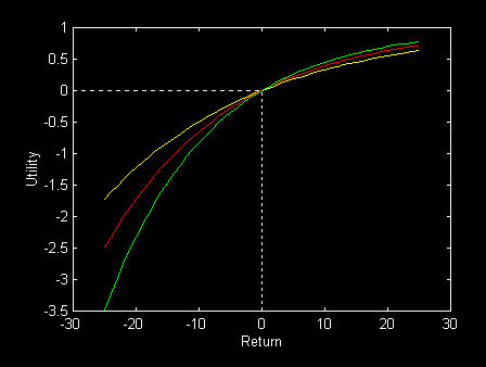
The figure below provides three examples of this function. We state return in percentage terms (e.g. 10.0 for an increase in wealth of 10%). As indicated, the utility associated with a return of zero is taken as zero, although no change in behavior would be implied if a constant were added to each such function. The flattest curve in the figure, shown in yellow, is based on a value of 0.04 for the parameter c. The next flattest (red) curve is based on a c value of 0.05, and the steepest (green) curve a value of 0.06.
In each case utility increases at a decreasing rate, exhibiting Investor risk aversion. Moreover, the greater the value of parameter c, the more curved the function and hence the more risk-averse the Investor in question.
To see the effect of curvature (c) on risk aversion, we can compute the certainty-equivalent return for a given distribution for our three Investors. Assume that Investment X offers a fifty percent chance of obtaining a return of 10% and a fifty percent chance of breaking even (i.e. obtaining a return of 0%). The expected utility of such a gamble will be:
eu = 0.5*(1-exp(-c*0)) + 0.5*(1-exp(-c*10))
We seek a return, rc, that will offer the same expected utility (which will, of course, be certain):
eu = 1-exp(-c*rc)
Combining the two equations produces the following relationship:
rc = -(1/c)*log(.5*exp(-c*0)+.5*exp(-c*10))
giving the following values for our three Investors:
     c        rc
    ----    ------
    0.04    4.5033
    0.05    4.3814
    0.06    4.2610
Even though the expected return from the investment is 5.0%, all three of these Investors will accept a smaller amount for certain to give up the investment. However, the amounts differ. The Investor for whom c=0.04 would be indifferent between the investment in question and 4.5033 percent for certain. The second Investor would be willing to accept a lower certain return (4.3814 percent), reflecting greater risk aversion. The third Investor, even more averse to risk, will accept even less (4.2610 percent) in return for giving up the investment. The greater is parameter c, the greater is the Investor's risk aversion.
The negative exponential utility function is especially convenient in a world of normally-distributed outcomes. Recall that expected utility is the integral of the utility function using the probability distribution as weights. If the former is negative exponential and the latter is normal, it will be the case that expected utility will be a simple function of the mean and variance of the distribution:
eu = e - (v/t)
Here, e is the expected outcome, v is the variance of the outcome, and t equals (2/c), where c is the parameter from the investor's utility function. For our three Investors:
    c       t
   ----    ----
   0.04    50.0
   0.05    40.0
   0.06    33.3
Parameter t measures the Investor's risk tolerance. Not surprisingly, the greater an Investor's risk aversion (c), the smaller is his or her risk tolerance (2/c).
If the probability distribution of returns is not normal, the expected utility of an investment for an Investor with a negative exponential utility function is likely to differ somewhat from that given by the simple mean-variance formula. For example, consider the investment with a 50/50 chance of returning 0% or 10%. It offers an expected return of 5%, a standard deviation of 5% and a variance of 25. The distribution is far from normal. Nonetheless, the (e-v/t) formula provides good approximations even in this case, as can be seen by comparing its values with the exact certainty-equivalents calculated earlier for our three Investors:
     t      exact    approx
   ----    ------     -----
   50.0    4.5033     4.500
   40.0    4.3814     4.375
   33.3    4.2610     4.250
Although the formula provides only approximate values when the distribution of returns is non-normal, it may nonetheless give very good approximations in such cases.
Of course these statements rely on the assumption that an Investor's utility function is in fact negative exponential, which need not be the case. However, if we assume that in the region near the selected initial point, the Investor's utility function can be adequately approximated by a negative exponential function, we can continue to use (e-v/t) to measure the desirability of a portfolio for the Investor in question. This could be termed a certainty-equivalent, as before. However, such a local approximation to the Investor's utility function is unlikely to hold over a large enough region to make the true certainty-equivalent equal this value. Hence we will term (e-v/t) the portfolio's expected utility or simply, its portfolio utility:
pu = e - (v/t)
Portfolio utility depends on both portfolio characteristics and the risk tolerance of the Investor in question. To emphasize this one could write:
pu(p,k) = e(p) - v(p)/t(k)
where e(p) is the expected value (or return) of portfolio p, v(p) is its variance, t(k) is Investor k's risk tolerance, and pu(p,k) is the utility of portfolio p for investor k.
Portfolio utility is measured in the same units as e. Consider the set of all portfolios that provide a given level of utility, say pux. All such portfolios must satisfy the equation:
pux = e(p) - v(p)/t(k)
or:
e(p) = pux + (1/t(k))*v(p)
In a diagram with mean (e) on the vertical axis and variance (v) on the horizontal axis, such an indifference curve will plot as an upward-sloping straight line, the intercept of which will indicate the associated portfolio utility. The slope of such a line indicates the rate at which the Investor is willing to trade expected value (or return) for variance. But the slope is 1/t(k). Thus t(k), the reciprocal of this slope, is the rate at which the Investor is willing to trade variance for expected return. Indeed, we can define t(k) as Investor k's marginal rate of substitution of variance for expected value.
If an Investor's risk tolerance were the same at all points in a mean/variance diagram, his or her indifference map would be a family of parallel lines, as shown below:
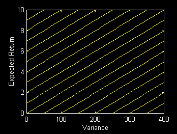
In fact it is unlikely that risk tolerance is constant over wide ranges of outcomes. However, we can infer its level from the choice of a prototypical asset mix, then assume that it is constant in the near neighborhood of the mean and variance of that mix.
Assume that the riskless rate of interest is 4% and that by investing in a diversified stock index portfolio it is possible to obtain an expected excess return over the riskless investment of 6% per year, with a standard deviation of 15% per year. If an amount x is invested in the stock index and an amount (1-x) in the riskless asset the return will be:
R = x*Rs + (1-x)*rr
where Rs is the return on the stock index and rr is the return on the riskless asset.
The expected return of the combination will be:
e = x*Es + (1-x)*rr
where Es is the expected return on the stock index.
Since the riskless asset has no risk, its standard deviation of return is zero. Hence the standard deviation of the combination will equal that of x*Rs. Examination of the formula for computing a standard deviation shows that the standard deviation of a positive constant times a variable will equal the constant times the standard deviation of that variable. Hence:
s = x*Ss
The net result of these relationships is that a combination in which x is invested in the stock index and (1-x) is invested in the riskless asset will lie at a point on the straight line that connects the points plotting the two assets in mean/standard deviation space. If x = 0 the point will coincide with that of the riskless asset. If x = 1, it will coincide with that of the stock index. If x is between 0 and 1 the point will plot on the line between the two asset's points. If x is greater than one, it will plot on the extension of this line above the point representing the risky asset. The figure below shows the relationship for the case in question.
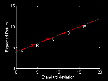
The portfolios shown in the diagram have the proportions:
         x    1-x
        ----  ----
   A     0    100
   B    25     75
   C    50     50
   D    75     25
   E   100      0
In this case the opportunity set (feasible region) is the straight line connecting the points. Since every feasible combination is efficient, the efficient frontier is the same line. Presumably there are other combinations of individual securities that lie below this line, but they have been excluded from the analysis. In any event, the frontier in this case can be described by the equation:
e = 4 + (6/15)*s
Now consider the same relationship plotted in a mean/variance diagram:
e = rr + (6/15)*sqrt(v)
In terms of e and v, the equation is non-linear, as shown in the figure below:
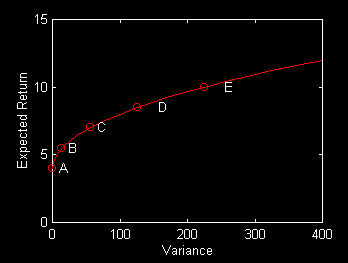
A relationship that plots as a line in mean/standard deviation space will plot as a curve that increases at a decreasing rate in a mean/variance diagram, as in this case.
Assume that Investor I has been presented with the implications of policies A,B,C,D and E for his or her standard of living in retirement. After careful reflection, C was chosen. Assume moreover that a finer set of choices (e.g. between B and D) was presented and C was again chosen (or that the Analyst is willing to assume that such would have been the case had the further analysis been undertaken). In any event, we know that one of Investor I's indifference curves is tangent to the frontier at point C and must therefore have the same slope as the frontier at that point, as shown below:
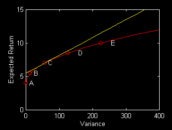
In this case:
e = 4 + (6/15)*(v.^(1/2))
thus:
de/dv =(1/2)*(6/15)*(v.^(-1/2))
or:
de/dv = (1/2)*(6/15)*(1/s)
Since the chosen point has a standard deviation of 7.5, the slope of the frontier at that point is:
(1/2)*(6/15)*(1/7.5)
or
6/225
The reciprocal is, of course, the Investor's risk tolerance. We thus infer that:
t(k) = 225/6 = 37.5
Note that the riskless rate of interest does not appear in this calculation -- only the expected excess return and standard deviation of the risky asset.
For further analyses we may assume that risk tolerance is constant in the near neighborhood of this point, as shown below:
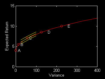
While it is convenient to show the derivation of risk tolerance from a choice of investment in mean/variance space, it is more intuitive to examine the situation in mean-standard deviation space, as in the following figure.
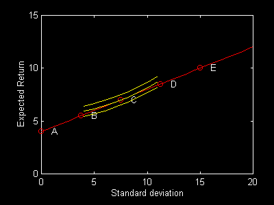
In this more familiar setting the efficient frontier plots as a straight line and each indifference curve increases at an increasing rate. Of course the point of tangency represents the same portfolio as before. Here too, the indifference curve and efficient frontier have the same slope (in this case, de/ds) at the chosen point.
In these diagrams we have shown only a limited range for the inferred indifference curve and for a few others with the same risk tolerance -- all within the near neighborhood of the chosen efficient risk/return combination. This was done to emphasize the fact that the Investor's actual indifference curves may differ considerably in areas of the diagram that are far from the chosen point. However, for relatively modest changes in the opportunity set (feasible region) it may be perfectly acceptable to assume that the fitted indifference curves reflect the Investor's true preferences. In such instances one can simply search the new opportunity set for a new point of tangency with the set of indifference curves with the same risk tolerance as found in the initial study.
If the efficient portfolio is linear in mean/standard deviation space, there is a one-to-one mapping between risk undertaken and risk tolerance, assuming efficient investment strategies are utilized. Let the efficient frontier be:
e = a + b*s
then:
s = (e-a)/b
and
v = ((e-a)^2)/(b^2)
The rate at which v can be substituted for e along the frontier is thus:
dv/de = 2*(e-a)/(b^2)
For an investment strategy to be optimal, this must equal the investor's risk tolerance t:
     t =  2*(e-a)/(b^2)
       = (2*(e-a)/b)/b
But s=(e-a)/b. Thus:
t = (2*s)/b
and
s = (b/2)*t
It follows that, compared with an "average investor":
     an Investor with twice the risk tolerance
     should take twice the risk

     an Investor with half the risk tolerance
     should take half the risk
Similarly:
     if Investor A optimally takes half the risk
     taken optimally by Investor B, then A has
     half as much tolerance for risk as B.
Note that this neat correspondence depends on the assumption that the efficient risk-return tradeoff is linear. In practice this is often approximately true, so the relationship holds to at least a first approximation.
While portfolio utility indifference curves plot as parallel upward-sloping straight lines in mean/variance space, they have a more familiar look in more intuitive mean/standard deviation ("return/risk") diagrams, as we have seen.
The equation for all combinations of e and s that provide a given level of portfolio utility pux is:
e = pux + (s^2)/t
Note that e is a quadratic function of s, and that:
de/ds= 2*s/t
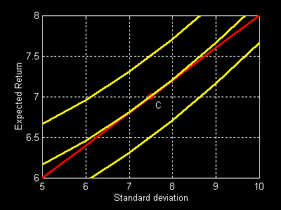
Hence such a curve increases at an increasing rate as s increases. Moreover, all such curves have the same slope for a given value of s, as can be seen from the equation and inspection of the following enlarged version of the area near the chosen point in the previous diagram:
In a later section we will show that efficient frontiers will always increase at a non-increasing rate in mean/standard deviation space. More simply put, they will either be linear or increase at a decreasing rate. Since our assumed indifference curves increase at an increasing rate, this assures that one and only one efficient combination of risk and return will, in principle, be optimal in every case. It should, however, be said that in practice Investors often find it difficult to make a single choice from among alternative efficient combinations, indicating that preferences are not as neatly defined as our expected utility theory would suggest.
In a one-period analysis it seems natural to measure outcomes in terms of end-of-period portfolio value, since this is a measure of wealth and, ultimately, consumption -- the source of utility. However, mean/variance analysis is seldom used in a strictly one-period setting. Rather, one derives a one-period portfolio utility function (more precisely, an Investor's one-period risk tolerance) from choices made in a multi-period setting (for example, as part of an asset allocation study). Although the connection between the formal one-period model and the selection of a multi-period strategy is somewhat inelegant, it is important to recall the context in which mean/variance analyses are in fact performed.
For this reason it is generally preferable to cast mean/variance problems in terms of portfolio return, as we have done. This makes it more likely that the Analyst can utilize the same risk tolerance from period to period, at least until circumstances change in significant ways.
To see this, consider an Investor with $100 in year 1 who chooses an asset mix with 50% invested in a riskless asset with a return of 4% and 50% invested in a stock index fund with an expected return of 10% and a standard deviation of 15%. Shown below are the opportunity set and the selected point in a diagram based on ending value (wealth).
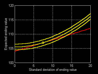
Now assume that in year 2 the Investor has a portfolio worth $110 and adds another $90 so that a total of $200 is available for investment. The new opportunity set in terms of wealth is shown below. Note that it has the same slope as the one for year 1.
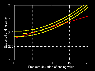
We know that the optimal mix lies at a point at which one of the Investor's indifference curves has the same slope as the opportunity set. But we have established that all indifference curves have the same slope for a given standard deviation. Since the new opportunity set is parallel to the old one, the Investor will choose the same standard deviation as before ($7.50). In this case, however, the associated mix will have only 25% invested in the stock index fund, which has a dollar standard deviation of $30.0 ($200*0.15). The dollar amount ($50) invested in the stock fund will, however, be the same as before.
Investors with constant risk tolerance stated in terms of end-of-period value will exhibit constant absolute risk aversion, keeping constant their absolute exposure to risky assets as wealth increases. Since this results in a decrease in their relative exposure to such assets, they exhibit increasing relative risk aversion. While some Investors might have preferences with such characteristics, most, will have greater risk tolerances expressed in value terms, as their wealth increases.
Consider now a portrayal of Investor preferences in terms of portfolio return, with risk tolerance indicating the Investor's willingness to trade variance of return for expected return. The figure below shows the situation in year 1. It also shows the situation in year 2. In such a situation, an Investor with constant risk tolerance expressed in terms of return would select the same relative mix of risky and riskless assets, no matter what his or her wealth -- behavior consistent with constant relative risk aversion.
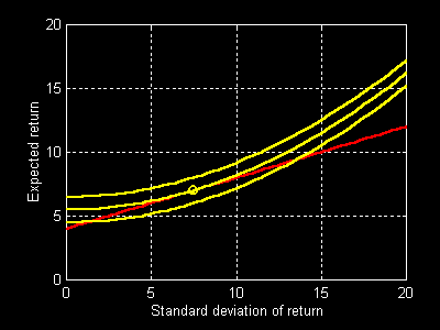
The assumption of constant relative risk aversion seems much closer to the preferences of most investors than does that of constant absolute risk aversion. Nonetheless, it is by no means guaranteed to reflect every Investor's attitude. Some may wish to take on more risk (standard deviation of return) as their wealth increases. Others may wish to take on less. Many Analysts counsel a decrease in such risk as one ages. Some strategies are based on acceptance of more or less risk, based on economic conditions. And so on.
For these and other reasons it is important to at least consider strategies in which an Investor's risk tolerance (vis-a-vis one-period return) changes from time to time. However, such changes, if required at all, will likely be far more gradual than those associated with a constant risk tolerance expressed in terms of end-of-period value.
Henceforth, unless stated otherwise, when we use the term risk tolerance, we will mean the Investor's marginal rate of substitution of the variance of one-period return for expected one-period return. Similarly, we will assume that portfolio utility is based on the expected return, variance of return and Investor risk tolerance based on one-period return. In cases involving zero-investment strategies we will sometimes be forced to deal in value terms. However, in such situations we will derive a utility function for end-of-period value from an assumed constant risk tolerance based on one-period return.
Some use the term risk-adjusted expected return or, more simply, risk-adjusted return, for the construct we have termed portfolio utility. We illustrate with an example:
     Expected return                    7.60     e
     Risk (standard deviation)          9.00     sd
     Variance                          81.00     v = sd^2
     Risk Tolerance                    45.00     t
     Risk Penalty                       1.80     v/t
     Risk-adjusted Expected Return      5.80     e - v/t
The expected return is 7.60%, but the investment has a risk of 9%. The Investor in question thus subtracts a risk penalty of 1.80% to obtain a risk-adjusted expected return of 5.80%. As stated earlier, the risk penalty depends on both the portfolio's risk and on the Investor's tolerance for risk. Other things equal, the greater the risk, the greater the risk penalty. And, other things equal, the greater the Investor's risk tolerance, the smaller the risk penalty.
The Analyst's main task is to find the portfolio with the maximum risk-adjusted expected return (portfolio utility) for the Investor in question. The figure below shows the relationship between (1) portfolio utility for an Investor with a risk tolerance of 45 and (2) the percent invested in the stock index fund in our previous example (a riskless return of 4% and a stock index fund with an expected return of 10% and a standard deviation of 15%). In this case it is optimal to invest 60% in the stock index fund and 40% in the riskless asset. The characteristics of this solution are those shown in the preceding table.
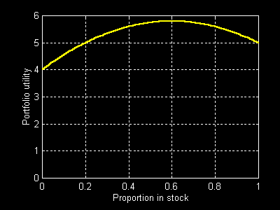
Not surprisingly the "utility hill" plots as a quadratic function of the proportion invested in the risky asset. The Analyst's goal is to place the Investor at the top of this hill.