Research: STM, Dr. Brian Moritz

Scanning Tunneling Microscopy (STM) is an experimental technique used to probe the physical surface and electronic structure of materials. In a typical STM experiment, a metallic tip is held a distance above the sample in high vacuum and a bias voltage is applied across the tip-vacuum-sample interface. This results in a tunneling current into or out of the sample that is proportional to the convolution of the density of states (DOS) of the tip and the sample. For a metallic tip the DOS is constant and so the current-voltage (I-V) curve's derivative is directly proportional to the DOS of the sample (multiplied by the relevant tunneling matrix elements). The point-like nature of the tip allows STM to probe the sample with atomic precision and the technique provides real-space information about the electronic structure of the sample.

Quasiparticle Interference

The real-space nature of an STM probe allows it to provide complementary information to momentum-resolved photon probes such as ARPES. However, the technique of Fourier Transform STM (FT-STM) has recently been developed, where momentum-space properties of a material are inferred from Fourier transforming its real space image. This technique has proved useful in studying the momentum-space structure of the high-T_c cuprate superconductors.

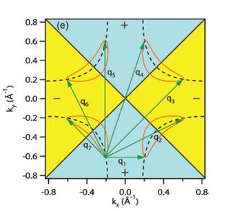
Fig 1: Schematic diagram of the QPI q-vectors from the octet model.

The elementary excitations of a superconductor are called ''Bogoliubov quasiparticles,'' which are a linear combination of an electron and a hole in opposite spin and momentum states. When quasiparticles scatter off of impurities in a material, their momentum-space eigenstates are mixed, which results in quasiparticle interference (QPI). This QPI produces a modulation of the material's real space density of states (DOS) and is hence detectable with STM. If Fourier transformed to momentum space, the modulation shows up as a set of peaks, which are interpreted according to the octet model. In this model, the maximum quasiparticle DOS occurs at the ends of ''banana shaped'' contours of constant quasiparticle energy that appear around the normal state Fermi surface. Due to the large joint DOS between the ends of these contours, quasiparticle scattering is dominated by seven momentum space vectors (q1, ..., q7) that connect the ends of these contours. FT-STM can be used to measure these q-vectors, and how they evolve with changing bias energy.

As bias energy is increased, some of the q-vectors grow, while others are suppressed upon crossing the antiferromagnetic zone boundary. The behavior of the various q-vectors can be explained by studying the momentum dependence of impurity scattering. This momentum dependence affects some q-vectors differently than others, because different vectors connect different parts of the Fermi surface. For example, some q-vectors connect Fermi surface locations where the phase of the superconducting gaps are equal, whereas others connect points of opposite phase.

We are performing calculations to compare to FT-STM data in order to study how the momentum dependence of the impurity scattering affects the various q-vectors, and compare the FT-STM results to data taken with ARPES. We are considering different types of scattering, for example, scatterers that modify the electron hopping parameter or the superconducting gap.

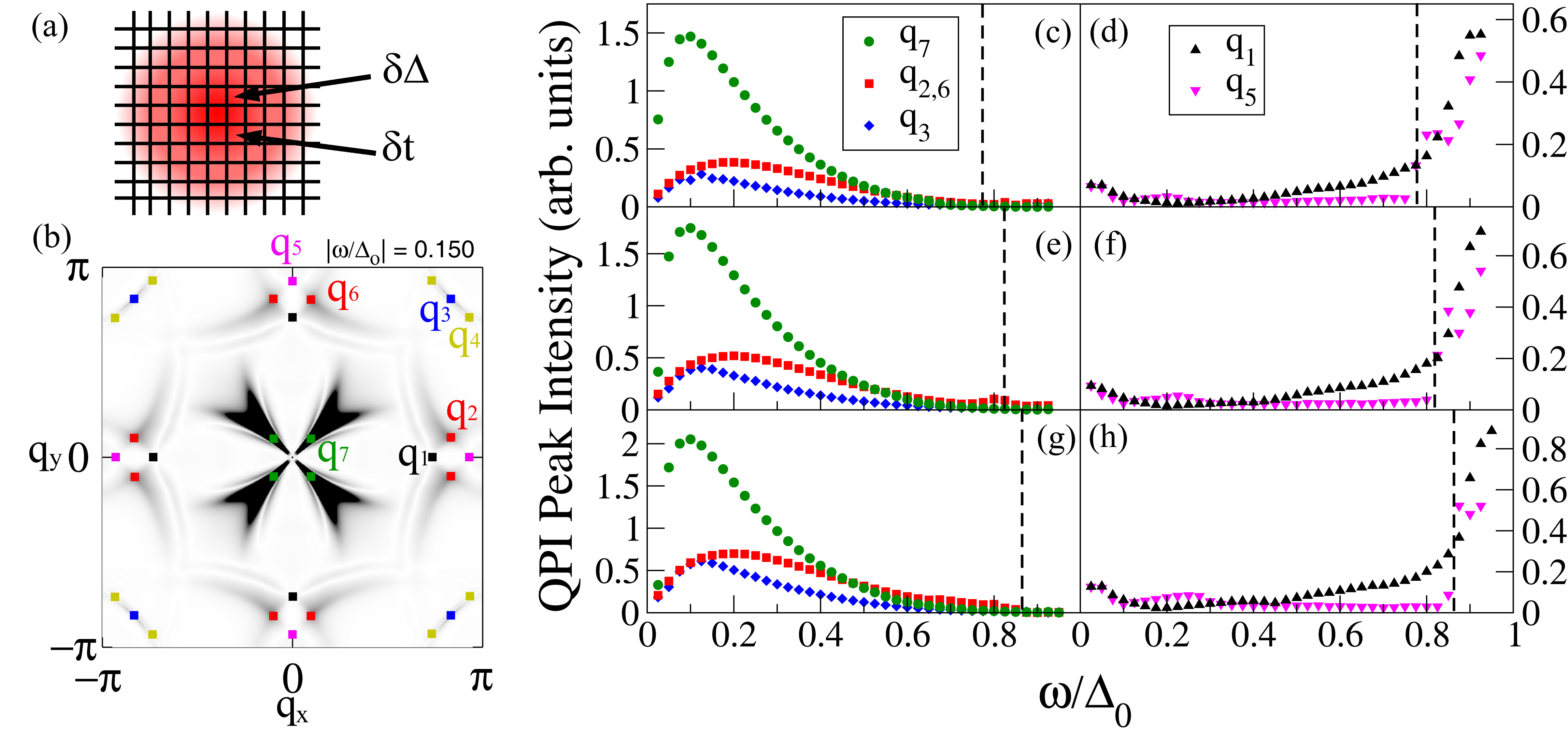
Fig 2: (a) Sketch of the patch used for calculations. (b) Z map for |ω/Δ₀|=0.15. The QPI wave vectors q₁ - q₇ are indicated. (c)-(h) QPI peak intensities determined from the Z map for 5% (c,d), 10%(e,f) and 15% (g,h) hole doping. (c),(e) and (g) show the intensity for wave vectors q₇, q_2,6 and q₃. The dashed line in each panel indicates the energy where the tips of the CCEs cross the antiferromagnetic zone boundary, where the peak intensities associated with q_2,3,6,7 vanish. (d),(f) and (h) show the intensities for wave vectors q₁ and q₅, which rise on approaching the antiferromagnetic zone boundary. From Reference 5.

One can suppress error due to tip alignment inaccuracies in STM experiments by studying Z-maps of the DOS, which is defined as the ratio of the DOS at positive bias to the DOS at negative bias. We also utilize a Z-map in order to make a meaningful comparison between our calculations and experiment. A movie of a Fourier transformed Z-map from our calculations is shown below. It shows the evolution of the Z-map and the corresponding peaks associated with each of the q-vectors as a function of applied bias voltage.