Research Discussions

The following log contains entries starting several months prior to the first day of class, involving colleagues at Brown, Google and Stanford, invited speakers, collaborators, and technical consultants. Each entry contains a mix of technical notes, references and short tutorials on background topics that students may find useful during the course. Entries after the start of class include notes on class discussions, technical supplements and additional references. The entries are listed in reverse chronological order with a bibliography and footnotes at the end.

Prological Epilogue

Usually an epilogue appears at the end of a book and a prologue at the beginning. However, the entries in this research log appear in reverse chronological order and so I've coined the phrase "Prological Epilogue" to refer to an epilogue that appears as a prologue to a text organized in reverse chronological order. This literary conceit serves in the present circumstances to note that the final class for this installment of CS379C occurred on June 1 and that all the later entries are included for students who continued working on their projects as well as new students who joined the group and started new projects. These students regularly met with me and my colleagues at Google and were provided with Google Cloud Compute Engine accounts to work with some of the larger datasets and take advantage of the machine learning resources enabled through the TensorFlow and TensorProcessorUnit technologies.

September 21, 2016

For the last few weeks I've been designing, building and experimenting with new tools for exploring the local structure of dense microcircuit connectomes. I spent yesterday developing a few demos to show off what I've done so far. The following notes are sketchy, but I'm hoping that the plots, associated captions and the introductory presentation I made during the San Francisco Neuromancer Rendezvous will provide enough context to give you an idea of what I'm trying to build.

This log entry emphasizes topological invariants as microcircuit features. However, more-traditional, graph-theoretic methods for identifying functionally-relevant patterns of connectivity in terms of network motifs may work equally well or better. In the following, you may be well served by focusing primarily on the figures and their captions, since the intervening text consists primarily of notes to myself for expanding this entry to provide a more complete account of this project.

Revise and summarize earlier notes on using topological invariants to investigate the structural and functional properties of local regions of densely reconstructed microcircuits [ … ] review reasons for turning to the FlyEM dataset from Janelia [ … ] enumerate some of the main advantages of using the extensive FlyEM metadata provided by Janelia, and, in particular, the opportunity it affords for testing automated analysis algorithms to infer function from structure. [ … ] ←

Figure 1: Much of the computation occurring in a neural circuit takes place in the synapses. This observation is particularly apropos in the case of recursive dendrodendritic¹ pathways[228], but applies much more broadly. Circuit (A) depicts a simple recurrent circuit in which two dendrites exchange information. Such exchanges need not result in an action potential being initiated in either of the two cell bodies. The locations of the respective cell bodies are not particularly relevant to the computations carried out in the region bounded by the two dashed red lines. We choose to characterize the locality of these computations as occurring entirely within the bounded region as illustrated in (C) rather than (B). Whether factors external to the bounded region influence the computations or the computations themselves influence external factors may not be apparent at the granularity assumed in this figure, but should become obvious at higher levels in a hierarchy of representations.

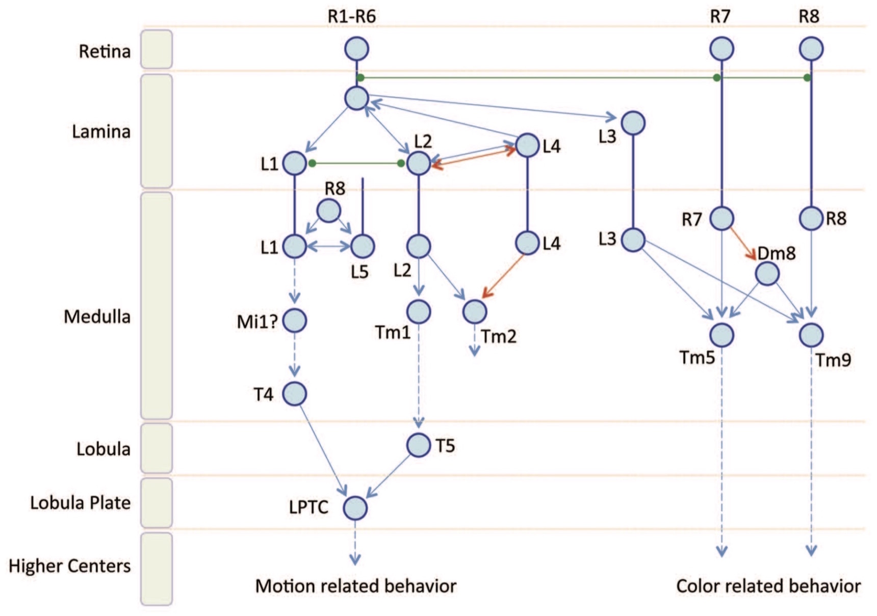
Mention related research at Janelia on the Drosophila visual system including, on the structural side, the work leading up to the seven-column medulla dataset [248, 281, 254], and, on the functional side, calcium imaging work out of Michael Reiser's lab [248]. Provide some detail on the resources offered in the FlyEM dataset and the extensive supporting tools and metadata. Note how the cell-type annotations and skeleton data facilitated much of the work described in this log entry.

Figure 2: This graphic shows the points that define the skeletons for the central-column medullar intrinsic (Mi1) neuron (shown in blue) and the six neighboring Mi1 neurons (shown in green) located in the six adjoining, hexagonally-arranged columns. Since there is exactly one such neuron per column and its processes are confined to and extend throughout the associated column, we can fit a line to each set of skeletal points to obtain axes for each of the seven columns featured in the Janelia seven-column-medulla dataset. The central-column axis is shown in red and the axes for the adjoining six columns are shown in yellow. [See Appendix A for an introduction to the visual system of the adult Drosophila Melanogaster.]

Mention Alexander Borst's research on the fly visual system [ … ] Borst and Euler [26] [ … ] possible relevance to the Reichardt-Hassenstein motion model which posits specific circuits including cell types that could be explained by or identified with topological properties [ … ] there are some obvious reasons why this would be challenging to achieve [ … ] thoughts about what constitutes localized computation [ … ] review of interpretations of topological invariants in the context of annotating neural circuits [51, 60, 89, 233] [ … ] ←

Figure 3: Fiducial landmarks like the columnar axes shown in Figure 2 serve to identify regions of particular interest. In this graphic, the distances from the central column axis (shown in red) to the soma of the six Mi1 neurons in the adjoining columns (where distance is depicted as a green line from the centroid of the soma to the axis) along with a sample of the distances (shown in green) to the soma of Mi1 neurons that adjoin the central seven. Using these distance estimates, we can define a cylindrical region of interest that includes the central seven but excludes the remaining columns and their respective neurons. We might also restrict interest to one or more of the ten layers of medulla.

Figure 4: Our objective is to characterize the local microstructure of neural circuitry. For each (spherical) subvolume obtained by a conventional sliding-window convolutional operator with fixed stepsize and diameter, we compute the directed flag complex [60] of the subtended graph fragment along with associated topological invariants, including the Euler characteristic and Betti numbers, to be used as features in subsequent analyses. The graphic shows a subgraph with green nodes and black edges along with a small sample of nodes drawn from the rest of the graph. The sample nodes are rendered as light-yellow, partially-transparent circles sans edges to avoid obscuring structural detail in the subgraph. A 4-simplex—one of many thousands in the subgraph—consisting of five nodes is shown highlighted in blue with red-font, cell-type abbreviations as labels and magenta edges with thickened lines to represent end points. The single sink of the 4-simplex is rendered as a square marker.

Figure 5: We scaled the coordinates of synapses within the restricted cylindrical volume—shown in Figure 3—to the unit cube and sampled spherical subvolumes 0.75 in diameter with a 0.50 stepsize generating 8K subvolumes and their corresponding coordinates[ … ] We computed the directed flag complex of each of subvolume and generated vectors of the form ⟨ Ε, Β₂, …, Β_K , Σ₂, …, Σ_K ⟩, where Ε is the Euler characteristic, Β_n is the nth Betti number, hmSigma is the number of n-simplices in the complex, K = 10 in the experiments reported here, resulting in a crude feature vector of length 17 for each subvolume. We cluster these vectors, assigning a different color to each cluster and plot the result using the 3D coordinates of the spherical subvolumes. [ … ] Create Juypter notebook with interactive version of this plot. ←

Appendix A: Drosophila Visual System

Expand this section and assign credit for the research and currated datasets alluded to in the borrowed figures. Provide the necessary background for students taking CS379C and supply links to the 2016 FlyEM Connectomic Hackathon and Virtual Fly Brain Project.

Figure 6: [ … ] Coronal cross-section of an adult Drosophila melanogaster highlighting one lobe of the Drosophila visual system. [SOURCE: the Virtual Fly Brain website using their 3D viewer and query tools]

Figure 7: [ … ] [SOURCE: the resources made publicly available by the Janelia FlyEM Project website]

Figure 8: [ … ] [SOURCE: the resources made publicly available by the Janelia FlyEM Project website]

Figure 9: A diagram of connectivity in the Drosophila visual system. The visual system relies on hundreds of repeated units, the visual columns, to process information across the visual field in parallel. Shown here are some known components of a single visual column and their inter-connectivity. Motion-related behaviors depend on the R1-R6 pathway to compute motion signals, while the R7/R8 pathway is responsible for color perception and color-related behaviors. In the diagram, each neuron is simplified to one or more blue circles, which also depict the sites of connections. The direct synaptic connections are shown as arrows. When direct connection is unknown, an arrow with a dotted line is used to indicate the flow direction of information. Reciprocal connections are shown as a line with two arrow heads. Electrically coupled connections via gap junctions are depicted as green lines with green circles. The red color arrows indicate synaptic inputs coming from other visual columns. Most connections in the diagram were only revealed by reconstruction of serial EM sections, and their functions have yet been studied or confirmed by electrophysiology or behavioral assays. [SOURCE: Yan Zhu, Laboratory of Brain and Cognitive Science; Institute of Biophysics; Chinese Academy of Sciences [282]]

August 5, 2016

If you don't have time to read Fischbach and Dittrich [73], the introduction provided in the 2015 FlyEM Connectome Hackathon is probably enough to get you going. If you have a fast network connection, there are a number of tools for exploring the seven-column medulla dataset. VirtualFlyBrain serves FlyEM data in responding to a wide range of queries, for example, here is the response to the query for "medulla intrinsic neuron Mi1". I also recommend reading [14] to accompany the earlier mentioned papers [248] and [254] providing the first analyses of this dataset.

The seven-column medulla dataset consists of connectome-graph information including a description of each neuron in neuronsinfo.json and each synapse in synapses.json plus morphological information in the directory ./skeletons/ consisting of one file for each neuron containing a skeleton representation of the neuron specified in SWC² file format:

One file for each skeleton such that each line of the file is of the form:
  
n T x y z R P

n is an integer label identifying the current point, & incremented by one from one line to the next.

T is an integer representing the type of neuronal segment, such as soma, axon, apical dendrite, etc. 

The standard accepted integer values are given below.

0 = undefined
1 = soma
2 = axon
3 = dendrite
4 = apical dendrite
5 = fork point
6 = end point
7 = custom

x, y, z gives the cartesian coordinates of each node.

R is the radius at that node.

P indicates the parent (the integer label) of the current point or -1 to indicate an origin (soma).

To organize the 3D Euclidean space in which the nodes of the graph—neurons—are embedded, the first thing we do is to transform the coordinates to a frame of reference more suitable for analysis, and then scale the coordinates to the unit cube to facilitate subsequent indexing and alignment. Ideally we would choose the centroid of the middle column as the origin of the new coordinate space and align the z-axis with the central axis of this column. Since the columns are fictional idealizations, we follow Stephen Plaza's suggestion to orient the frame of reference using the Mi1 medullary intrinsic neuron in the central (home) column since there is exactly one Mi1 type neuron per column and the cell is almost entirely contained within its associated column.

Below I've listed the neuronsinfo.json entry for the Mi1 neuron associated with the central column. The key 30465 is the cell body ID and is used to retrieve skeleton information stored in ./skeletons/30465.swc. PSD refers to post-synaptic dendritic spines, Tbar refers to the pre-synaptic boutons. Column PSD/Tbar Fraction lists the fraction of PSD/Tbar in each of the seven focal columns labeled A-F plus home or H, and Layer PSD/Tbar Fraction lists the fraction of PSD/Tbar in each of the 10 layers of the medulla. Column Volume Fraction lists the fraction of the cell arborization in each of the eight central columns. Note 30465 is almost entirely contained in H:

    "30465": {
        "Class": "Mi", 
        "Column ID": "home", 
        "Column PSD Fraction": {
            "A": "0.0163636364", 
            "B": "0.0145454545", 
            "C": "0.0018181818", 
            "D": "0", 
            "E": "0.0181818182", 
            "F": "0.0418181818", 
            "H": "0.8363636364"
        }, 
        "Column Tbar Fraction": {
            "A": "0", 
            "B": "0.0025125628", 
            "C": "0", 
            "D": "0", 
            "E": "0.0025125628", 
            "F": "0.0025125628", 
            "H": "0.9170854271"
        }, 
        "Column Volume Fraction": {
            "A": "0.001248788", 
            "B": "0.01323397", 
            "C": "0.0036433003", 
            "D": "0.0002563759", 
            "E": "0.005611789", 
            "F": "0.0087104412", 
            "H": "0.9085093161"
        }, 
        "Columnar Location": "Interior", 
        "Columnar Spread": "Single Columnar", 
        "Layer PSD Fraction": {
            "m1": "0.3732394366", 
            "m2": "0.1285211268", 
            "m3": "0.036971831", 
            "m4": "0.0052816901", 
            "m5": "0.2024647887", 
            "m6": "0.0158450704", 
            "m7": "0", 
            "m8": "0", 
            "m9": "0.1901408451"
            "m10": "0.0457746479", 
        }, 
        "Layer Tbar Fraction": {
            "m1": "0.1642156863", 
            "m2": "0", 
            "m3": "0.0147058824", 
            "m4": "0.0343137255", 
            "m5": "0.0637254902", 
            "m6": "0.0049019608", 
            "m7": "0", 
            "m8": "0", 
            "m9": "0.5294117647"
            "m10": "0.1789215686", 
        }, 
        "Name": "Mi1 H", 
        "Superclass": "Intrinsic Medulla", 
        "Type": "Mi1"
    },

To determine the origin of the transformed coordinate space, we compute the centroid of the skeletal coordinates supplied in ./skeletons/30465.swc. To normalize the coordinates, we scale each dimension to the interval [-0.5,0.5]. Stephen mentioned the column was somewhat tilted. We could fit a reference line to the 30465 skeletal coordinates and rotate the coordinate frame so the reference line coincides with the z-axis, but will refrain from mucking about further, unless the tilt in the original coordinate space unduly complicates analysis. Note we can use the Mi1 neurons associated with the other six focal columns to provide additional structurally-relevant spatial information to infer functional properties of cells.

Using the additional annotations available in synapses.json, neuronsinfo.json and ./skeletons.*.swc, we can enrich the language we use for defining functional motifs as Art suggested earlier this week. We can also use these annotations to evaluate motifs that rely entirely on directional connectivity available in the connectome adjacency matrix, and, given the functional data described in [248] which Michael Reiser has agreed to share with us, we might have a much better chance of aligning structural and functional information.

August 3, 2016

The number of ommatidia in a compound eye has a wide range, from the dragonfly with its ~30,000 ommatidia to subterranean insects having around 20. Even within the order of so-called true flies known as Diptera, there is wide variation, e.g., a fruit fly — Drosophila melanogaster — has ~800, a house fly ~4,000, and a horse fly ~10,000 ommatidia. The number of ommatidia is directly related to the number of columns in the medulla: There are as many columns in the medulla as there are cartridges in the lamina and as many cartridges as there are ommatidia in the eye. To estimate the number of neurons in seven columns of Drosophila medulla, multiply the total number of neurons in the medulla—approximately 40,000—by seven and divide by the total number columns—approximately 800 (40,000 × 7 / 800 = 350).

In response to my question about whether there exists calcium imaging data for Drosophila, Michael Reiser from Janelia (Reiser Lab) responded positively, and graciously volunteered to share the data from his 2014 paper [248] focusing on visual-motion sensing. Borst and Helmstaedter refer to this work in their paper [27] concerning motion-sensing circuits that exist in both fly and mammal. Here's what Michael had to say:

MBR: We did calcium imaging from the medulla, with a calcium indicator expressed in approximately all cell types. We did a pretty rudimentary analysis (PCA) in the attached paper, but that was good enough to show striking agreement between spatial patterns of neuronal activity and specific anatomical pathways. Clearly there is a lot more that could be done with that original data set, although in my lab we have moved on to imaging from individual cell types, one at a time (to get at the specific question of how directionally selective motion signals emerge from non-selective inputs). If you would be interested to dig deeper, I'll make sure we get the data from the 2014 paper to you.

For purposes, of visualization and possible alignment with the functional (CI) data that Michael volunteered to share with us, I wanted to get more precise information on the location of columns, layers, particular cell types, etc. Here is an email exchange with Stephen Plaza regarding the position of the "home" column in the FlyEM data:

TLD: Do you have the coordinates of the centroid and dimensions of the central (home or H) column in the same coordinate frame as the cell body locations are provided. The axis of the column appears to be parallel to the z-axis. Also could you tell me the units of the cell body coordinates / locations? It looks like the max separation (in z) is over 6000, and, since the size of an entire Drosophila brain is around 590 μm × 340 μm × 120 μm that probably argues for using the nanometer as the unit for expressing coordinates but I wanted to be sure.
SMP: Correct. The column axis is roughly z-axis aligned (there is a slight tilt). The voxel resolution of the original dataset is 10 × 10 × 10 nm. I believe the skeletons are in one-to-one correspondence with the source data. 60-micron spans for the neurons seem correct. The best way to estimate column dimensions / location / etc is to use the Mi1 neurons since they are one per column and run down the center. The home column Mi1 should contain an H indication.

The primary topic examined in Nèriec and Desplan [182] is the development of the Drosophila visual system, "from the embryo to the adult and from the gross anatomy to the cellular level [...] explore the general molecular mechanisms identified that might apply to other neural structures in flies or in vertebrates." Worthwhile reading or at least skimming to acquaint yourself with its content for future reference. Regarding circuits exhibiting feedback and interesting substructural motifs, the discussion and cited work in Ehrlich and Schüffny [65] provide some interesting examples, for example, the following graphic illustrates two models of a putative attractor-network model of associative memory in layers II and III of neocortex:

Miscellaneous loose ends: I've been trying to carve out some time to think more about the relationship between conversation and programming—specifically pair—two humans—or semi-automated programming—a computer and a human. Here are few thoughts: Recovering from a misunderstanding, resolving ambiguity or mitigating errors, all of these have their analogies to what goes on in debugging code, pair programming, altering your travel plans, correcting and following directions with or without the aid of the person who gave you the instructions in the first place, understanding recipes and modifying procedures to suit new applications or use cases.

"What is this supposed to do?", "Does that do the same thing as hitting the escape key?", "Is that like the mapping function in Python?", "I want to get there in time for dinner.", "Are you enjoying this conversation? Would you like to talk about something else?", "Is there someone else I could talk to in order to get this straightened out?", "You think I can expense this dinner?", ..., How would you tell someone how to replace a washer on the cold water faucet of the kitchen sink? How would it make a difference if they could take apart a car and put it back together so it worked, but didn't know a thing about plumbing?

In fact, a large fraction of human communication — for that matter, human-computer interaction — involves context setting and switching, judging the attentiveness or understanding of your conversational partner, judging the interest of your audience in giving a public lecture, etc. "are you following this?", "Are we still talking about the same thing?", "Are we looking at the same person?" Estimating your interlocutor's tolerance for talking about whatever topic you opened the conversation with: "Am I boring you?", "Would you rather talk about something else?".

A couple of weeks back, I talked with Gilad Bracha <gbracha@google.com> and Luke Church <lukechurch@google.com> about possible synergy of my vaporish programmers apprentice PA with their proto project of generating code by finding and adapting similar code. Yesterday, I had lunch with Steve Reiss <spr@cs.brown.edu> and talked about his prototype system for semantics-based code search S⁶ that addresses similar use cases. Finally, DJ Seo sent me his new paper which came out in in Neuron yesterday. He and his collaborators have made considerable progress since he visited a few months back and now have a basic prototype system up and running [222].

July 31, 2016

I've been working with three Stanford students—Rishi Bedi, Nishith Khandwala and Barak Oshri—to develop software for computing localized, topologically-invariant properties of connectome adjacency matrices. Instead of computing global properties of the complete connectome, i.e., the directed graph of all neurons (vertices) and synapses (edges), we compute properties of the subgraphs restricted to subvolumes that (together) cover (local-region-of-interest-width > step-size > 0) or tile (step-size = local-region-of-interest-width) the 3D volume embedding the full graph.

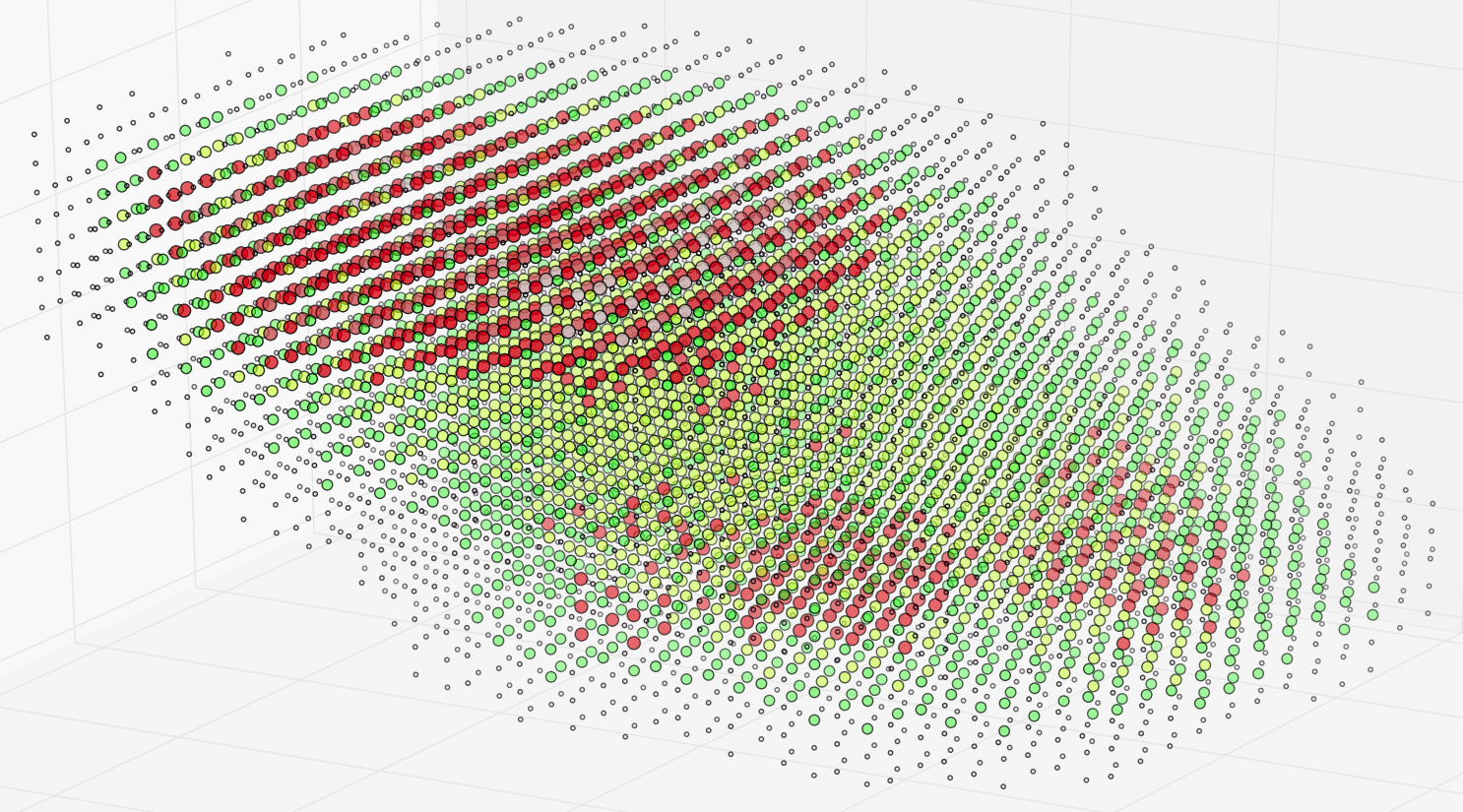
Until recently we worked with synthetic models from Costas' Anastassiou's and Henry Markram's labs at AIBS and EPFL respectively. These models may not exhibit biologically accurate circuits since they were generated probabilistically from distributions estimated by combining a wide array of published data [9, 166, 208]³. For example, the following plot shows a suspiciously-regular, synthetic cortical column consisting of approximately 20,000 neurons and 500,000 synapses:

Recently we've been working with the Janelia seven-column drosophila medulla dataset because (a) it is a relatively-large, well-curated dataset with high-quality reconstructions and detailed information about synapses, (b) it roughly corresponds to the same circuits we were looking at in the mouse visual system, and (c) it is more likely to provide us with a challenging test of our ability to automatically identify functionally similar regions of a large neural circuit using well-studied, spatially-mapped functional and structural designations.

If you're interested in learning about drosophila vision, these two review articles [25, 282] provide a good overview of the state of knowledge concerning the neural circuits implementing the fly visual system and related motion- and flight-control systems. Alexander Borst's website on the fly visual system at the Max Planck Institute is a great place to start for a quick introduction. The Janelia FlyEM website has lots of practical detail about how the data was collected and annotated, e.g., a set of rules used to classify neurons along with exceptions.

Takemura et al [254] review the work of several Janelia labs—including those of Lou Scheffer, Ian Meinertzhagen and Dmitri Chklovskii—analyzing the preliminary, semi-automated connectomic reconstruction of a portion of the seven-column medulla dataset, consisting of 379 neurons and 8,637 chemical synaptic contacts. This dataset continued to evolve and a somewhat larger set was featured in the 2015 Connectome Hackathon is available at FlyEM for download. The hackathon dataset includes 462 neurons and 53,383 (mostly chemical) synapses that, in the case of drosophila, have an unusual structure called a T-bar studded with multiple locations that make contact with post-synaptic neurons.

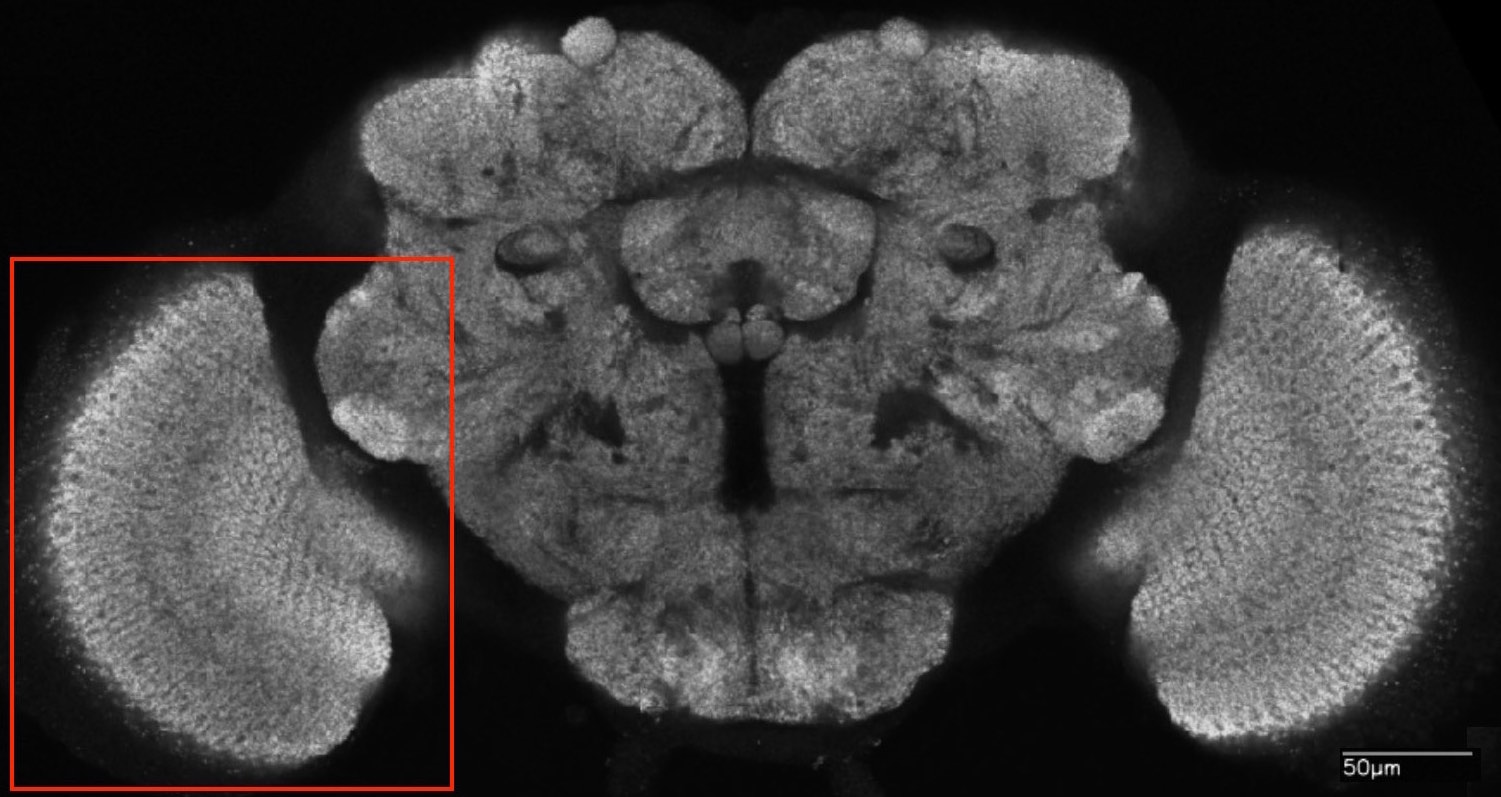
There is reason to believe that these highly-conserved regions of the drosophila brain are more stereotypical than the analogous regions of the mammal visual system. The primary components of this system consist of the lamina, medulla, lobula and lobula plate, including around 60K neurons—two thirds of which are located in the medulla, and representing a significant fraction of all drosophila neurons, usually estimated at around 150K [46]. As in mammalian cortex, the medulla is divided into several layers—ten in the case of drosophila—two of which have complicated local circuits consisting of inhibitory and excitatory interneurons.

There is a substantial literature focusing on the circuit-level function of the medulla and its neighboring visual areas. For example, Duistermars et al [62] provides interesting detail on the role of binocular interactions in flight, emphasizing the "interplay of contra-lateral inhibitory as well as excitatory circuit interactions that serve to maintain a stable optomotor equilibrium across a range of visual contrasts". Olsen and Wilson [189] provide insight into how genetic screening, optogenetic and pharmacological perturbations and modern imaging technology are being combined to map functional connectivity in the related areas and determine "causal relationships between activity and behavior".

Our initial experiments using the same code that we employed in analyzing the Anastassiou synthetic cortex data were disappointing. In the same regions where we would find subgraphs in mouse data consisting of hundreds or even thousands of neurons and ten times that many connections and exhibiting interesting topological motifs, the subgraphs in the fly data were small and structurally uninteresting. Initially, this didn't seem consistent with the analysis in Takemura et al [254]—for example:

The problem was that, although there were interesting circuits involving synapses linking axonal and dendritic arbors in the subvolumes corresponding to these graphs, the cell bodies (soma) were not located in these subvolumes. We store all the cell bodies in a KD tree and retrieve only those cell bodies that fall within a target subvolume to construct the corresponding subgraph G = { V, E }. The set of vertices V is just the set of neurons associated with the retrieved cell bodies. An edge (synapse) is in E if and only if the pre- and post-synaptic neurons are in V.

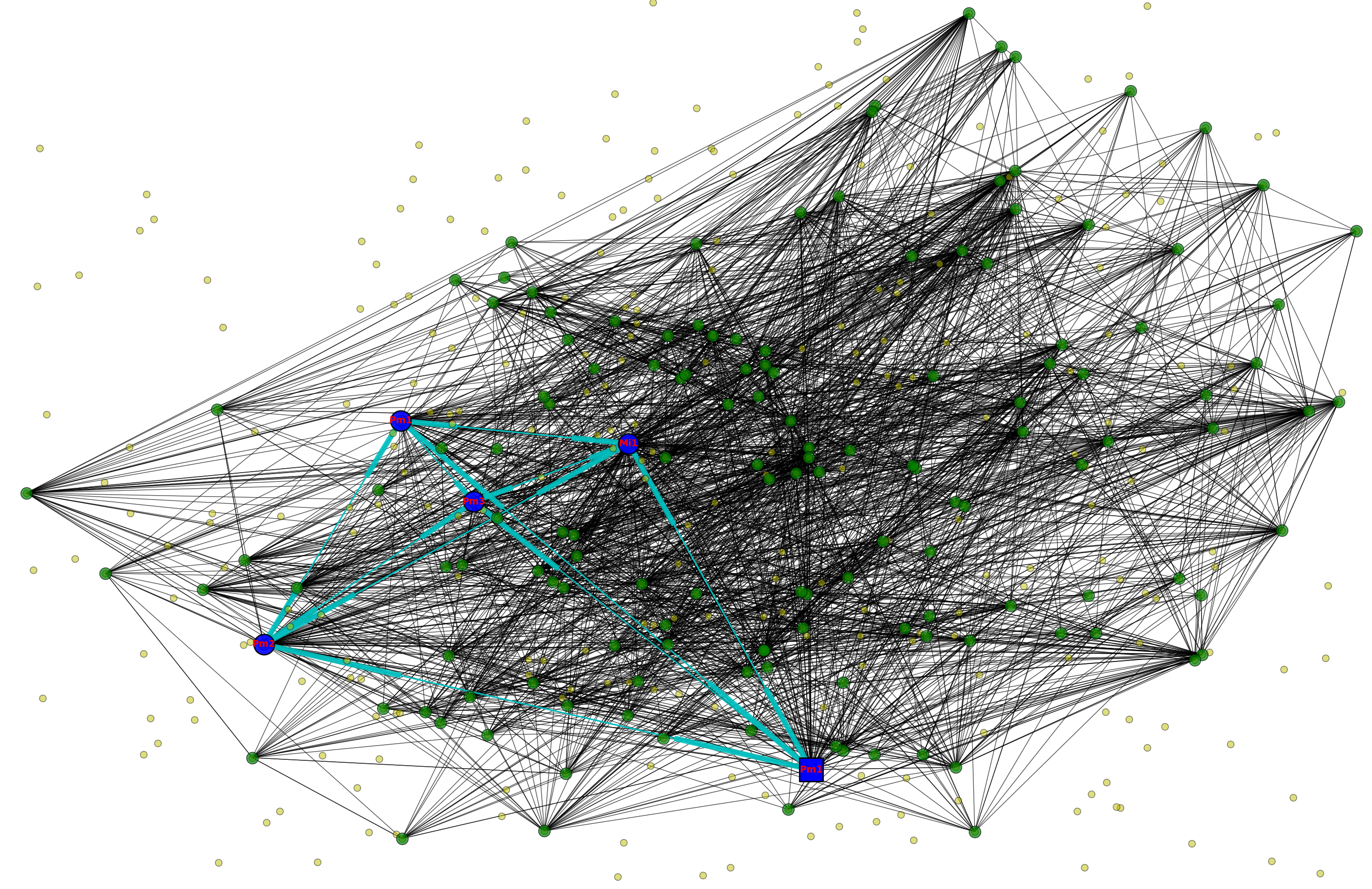
Note that, according to this rule, we can add an edge between n₁ and n₂ even when the all the synapses connecting n₁ and n₂ are located outside of the subvolume. We modified the rule so that, instead of storing cell bodies, we store all the synapses indexed by location and add an edge between n_PRE and n_POST irrespective of whether the location of either cell body falls within the subvolume. For example, in the figure below, the dashed green line bounds a subgraph that exhibits a 3-simplex as shown despite the fact that only B of the three cell bodies is located within the subvolume:

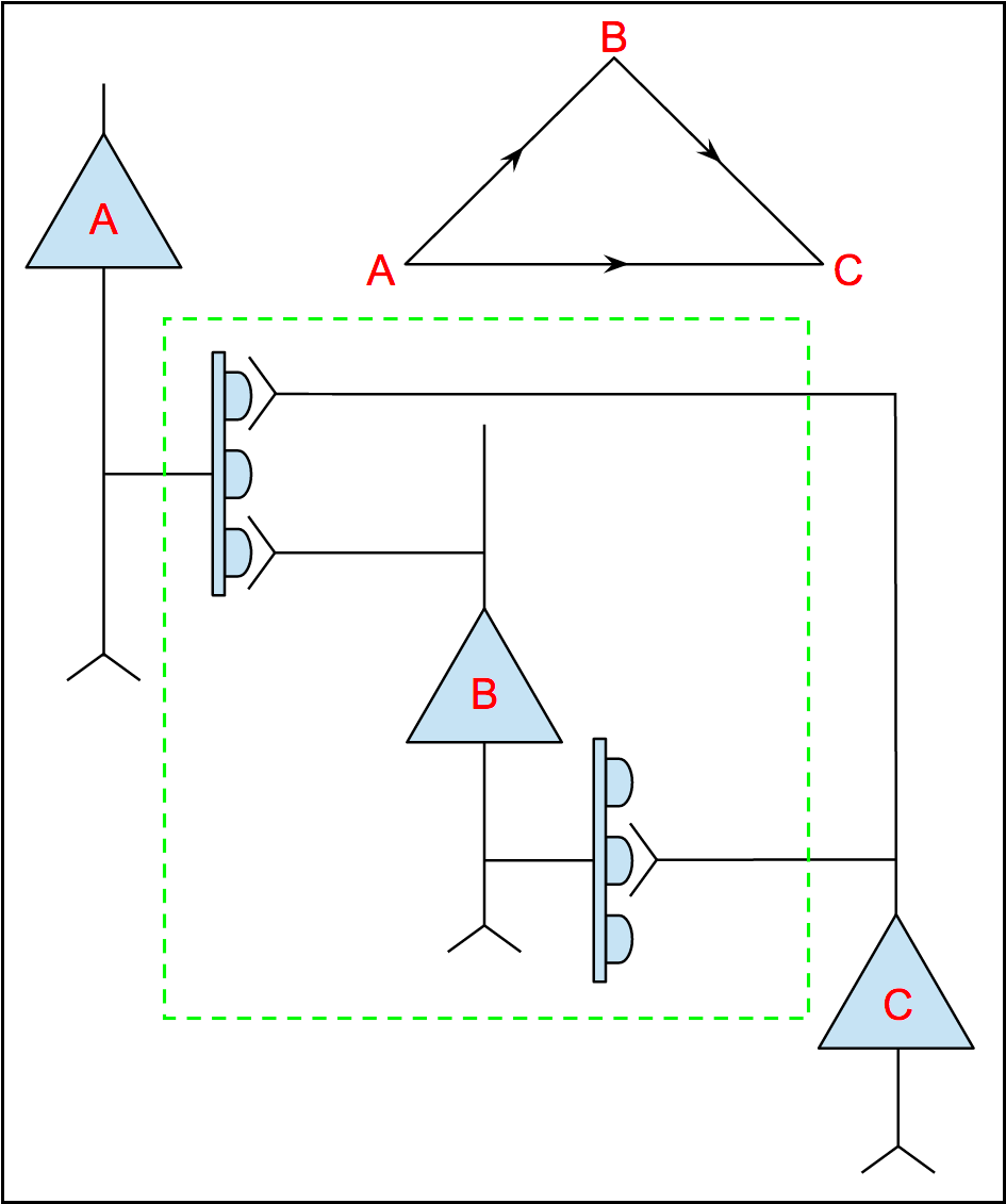The graphical conventions for drawing circuit schematics shown here are not standard, but, as I found out, there really is no widely-agreed-upon standard, a state of affairs leading to a good deal of confusion. It suffices in this case to know that synapses—generally T-bars in the case of the drosophila visual system—emanate from the axonal arbor of the pre-synaptic neuron. If you are interested in the debate over conventions for neural circuit schematic drawings you might be interested in this paper by Konagurthu and Lesk [146]. If you have more-realistic examples of 3-simplices, please share.

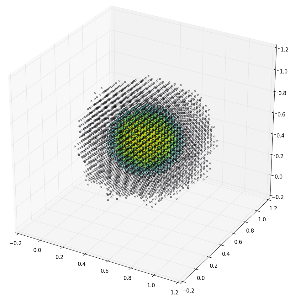
With this change in our definition of what constitutes an edge in a subgraph embedded in a given subvolume, we obtain a rich set of features that we can use in attempting to segment a connectome into functionally different regions. Here is a simple example in which we divide a unit cube enclosing the scaled coordinates of 50,000 synaptic (T-bar) loci into 1,000 subvolumes and, for each of the 1,000 associated subgraphs, compute a vector of topological features including those described in Dlotko et al [60] and cluster the vectors to produce the following graphic:

Miscellaneous loose ends: Look at the paper by Niepert et al [186] on a convolutional method for extracting and analyzing locally-connected regions of large graphs and and learning convolutional neural networks to classify such graphs according to various criteria. Read Ehrlich and Schuffny [65] on the touted novelty and relevance of published work on biologically-plausible network motifs.

June 1, 2016

Thanks to David Sussillo for the discussion at lunch today on inferring dynamical systems from aligned neural and behavioral data, and for the references to related work he recommended. Recall that David mentioned Omri Barak as someone else doing interesting related work in this area. Also remember that David's slides and the audio for his talk in class are available here and the class presentations from Saul and Andy are also on the course calendar page here if you want to review the material on C. elegans. The BibTeX entries are in the footnotes⁴

May 31, 2016

Here is some background information that I meant to send around earlier:

From talking with Clay Reid, Michael Buice and Jerome Lecoq, it looks like it will be another year and a half before we have aligned functional (CI) and structural (EM) data. There will likely be more experiments, variation in stimuli and annotation than we initially hoped for, but it will arrive later than expected. The bonus for waiting will include visualization tools, extensive annotation and careful curation. Depending on Neuromancer's priorities, we may be able to devote some cycles to expediting the image-processing requirements.
From talking with this same crew, I learned that the first installment of CI data is now available. The yield — number of neurons expressing the indicator — and coverage — number of neurons actually imaged — are disappointing, but will improve with Jerome's new microscope. You can learn most everything I know about the soon-to-be-released data from my notes following the Neuromancer rendezvous in Seattle last month, which you can find here if you want more detail.

When we met last week, we agreed to do the following exercise: the CI data is a 4D matrix s.t., for every x, y, z and t, we have a scalar whose value is an estimate of fluorescence at location (x, y, z) and time t. In fact, we'll have a raster representation with individual recordings for each neuron, but for now, think of the data as a 4D volume or, if you prefer, a 3D movie. Any sub-volume of the data corresponding to a four-dimensional hyper-rectangle represents the activity of a subset of the recorded neurons in carrying out a computation.

The only thing we know about the physical location of these neurons — in the current AIBS experiments GECIs are only expressed in the soma — is that if the 3D coordinates of the traces are close to one another then the neurons or at least the cell bodies are close to one another in the tissue sample. Without the morphological, genomic and proteomic information we will eventually get from the Allen Institute, we don't know a neuron's cell type, the circuits it is a part of, or the nature of its connections with other neurons⁵. What might we be able to infer about a sub-volume?

We could easily be looking at a sub-volume that represents but a fragment of anything one might recognize as a complete circuit. For example in our computer-chip analogy, we might be looking at the part of a multiplexer that performs the function of routing the selected inputs but is completely missing the part does the address decoding. Of course this begs two questions: (i) "Could we infer the function of the multiplexer if we were lucky enough to have selected the entire multiplexer circuit?" and (ii) "What's wrong with decomposing the circuit into separate addressing and routing circuits?"

I asked Semon and David to think about the problem as an image or video segmentation problem, and, in particular, come up with operators for performing the functional analog of boundary prediction. With the usual disingenuous warning that I didn't think very carefully about this, here are some observations — in the following, assume we treat each sub-volume as a multivariate time series. During our lunch conversation, we briefly discussed the idea of interestingness operators and I mentioned that the only coherent instantiations of this notion I know of make use of ideas from information theory, e.g., relative entropy also known as Kullback-Leibler divergence or some variant of Kolmogorov complexity — see Ahmed and Mandic [3].

The challenge in applying such ideas in practice generally comes down to finding a tractable algorithm. This often involves using tools from compressive sensing — see Yuriy Mishchenko [177], variants of Lempel-Ziv compression algorithms — see Ke and Tong [135], and sparse-coding and blind-source separation such as projection pursuit — see Aapo Hyvärinen [118]. I've also been thinking about indirect methods of measuring complexity that involve first fitting a general purpose RNN — perhaps a spiking neural network model like liquid-state machines [159] — and then estimating its complexity.

May 29, 2016

If your final project has hit a terminal snag and you despair of reviving it in time to meet the submission deadline, here's an alternative in the form of a research review paper that you might want to consider: Periodic discoveries of new types of neural structure and function continue to disrupt the field of neuroscience, threatening current theories that attempt to account for neural function. The project involves looking carefully at one such potential disruptive discovery.

Recently we learned about two mechanisms hypothesized to be relevant to both learning and neurological disorders including autism, Alzheimer's and Parkinson's. I'm referring to recent discoveries that the brain has its own immune system involving microglia and perhaps astrocytes, and that the neuritic plaques—extracellular deposits of amyloid β—and neurofibrillary tangles symptomatic of Alzheimer's and early onset senility might also be implicated in fending off infection.

The evidence is still inconclusive but there are some basic observations we can make about both microglia and amyloid β and I'd like you to try to sort out what we know from what has been published and speculated. Some believe that microglia play an important role in managing dendritic spine growth and hence in development and learning and therefore may have something to do with autism.

Specifically, I'd like you to search the literature concerning the dual roles of both microglia and amyloid β. Your project is to select and read carefully a few particularly relevant papers, summarize the most credible current theories and findings, and—most directly relevant to CS379C—reflect on to what degree we may have to account for these factors in a computational model of neural function in healthy organisms.

I've included below two recent papers—one for the findings concerning the negative role of microglia and the other concerning the potentially positive role of amyloid β that have made the headlines and are generally acknowledged by scientists to be credible if only preliminary at this stage:

Amyloid-β peptide protects against microbial infection in mouse and worm models of Alzheimer's disease. Science Translational Medicine 25 May 2016: Vol. 8, Issue 340, Pages 340-372. (LINK)
Microglia mediate early synapse loss in Alzheimer mouse models. Science 31 Mar 2016: Issue 000, Pages 000-000. The Rogue Immune Cells That Wreck the Brain (LINK) Alzheimer's may be caused by haywire immune system eating brain connections (LINK)

You can also find an entry in my class course notes (here) concerning microglia and their potential role in addiction and congenital autism. You might also give some thought to whether microglia—which appear to ubiquitous throughout the central nervous system—might provide some delivery vector or reporting mechanism for whole-brain recording. One potential problem is that they move around a lot, and so, while a scanning two-photon excitation and fluorescent-labeling method might enable dense reporting of local field potentials, the locations reporting might be different on each scan.

May 27, 2016

We discussed earlier how one might parallelize Algorithm 1 listed in the Supplementary Information section of [60] that generates the Hasse diagram of the directed flag complex associated with a given directed graph representing the connectome of a microcircuit. In this entry, we consider how to parallelize a multi-scale convolutional variant of the algorithm, and, in particular, how to compute feature-vectors consisting of topological invariants from local subgraph/subvolume regions of the microcircuit coordinate space so as to expedite the basic sliding-window algorithm used in applying linear filters and implementing convolution operators. We mention in passing how one could add a pooling layer that would smooth feature vectors over neighboring subvolumes, making it easier to segment large tissues into meaningful functional / computational components.

Figure 1: An illustration of the basic mathematical entities involved in computing topological invariants, including (a) the input corresponding to the directed graph of the microcircuit connectome, and (b) the output corresponding to the Hasse diagram representing the directed flag complex of the input graph. The graphic was adapted from Figure S5 from Dlotko et al [60].

I found the direction of the edges in the above depiction of the Hasse diagram confusing for two reasons: First, the edge, 123 → 12, is awkwardly understood as "the 2-simplex 123 has the 1-simplex 12 as a face", while 12 → 123, is naturally interpreted as "the 1-simplex 12 is a face of the 2-simplex 123". Second, the latter is consistent with the level-by-level construction of the Hasse diagram as described in Algorithm 1, starting with smallest simplices—the vertices of the graph—and working toward larger ones. In any case, I'm going to assume that the edge directions are reversed in the following discussion of how the Hasse diagram can be reused to expedite multi-scale convolutional persistent homology. If this not true in the current implementation, it can easily be remedied.

Let G = { V, E } be a directed graph with vertices V and edges E, and H = constructHasseDiagram(G) correspond to the Hasse diagram for the graph G—representing the microcircuit connectome. Create a spill-tree T to enable fast (parallel) retrieval of subsets of the 3D-indexed vertices of G—see [154, 153, 155] and the slide-deck presentation by Dafna Britten (PDF) for technical details. For the purpose of this discussion, let U = subsetSpillTree(T ,V, X_i, Y_i, Z_i, Width, Height, Depth) return the subset U of all the vertices in V whose coordinates are contained within the 3D region of size Width × Height × Depth located at ⟨ X_i, Y_i, Z_i ⟩.

Let { BN, EC } = computeBettiEuler(U, H) compute the Betti numbers BN and Euler characteristic EC for the subgraph G_U defined by U ⊆ V together with edges E_U ⊆ E such that u_i → u_j ∈ E_U if and only if u_i ∈ U and u_j ∈ U. The function computeBettiEuler works by constructing the Hasse diagram for G_U such that calls to the function computeHomology(H_U) return the Betti numbers BN and Euler characteristic EC for H_U as is done in Pawel's code. We construct H_U from H as follows, assuming—as explained above—that the directed edges in H are reversed, i.e., edges in H point from k-simplices to (k + 2)-simplices.

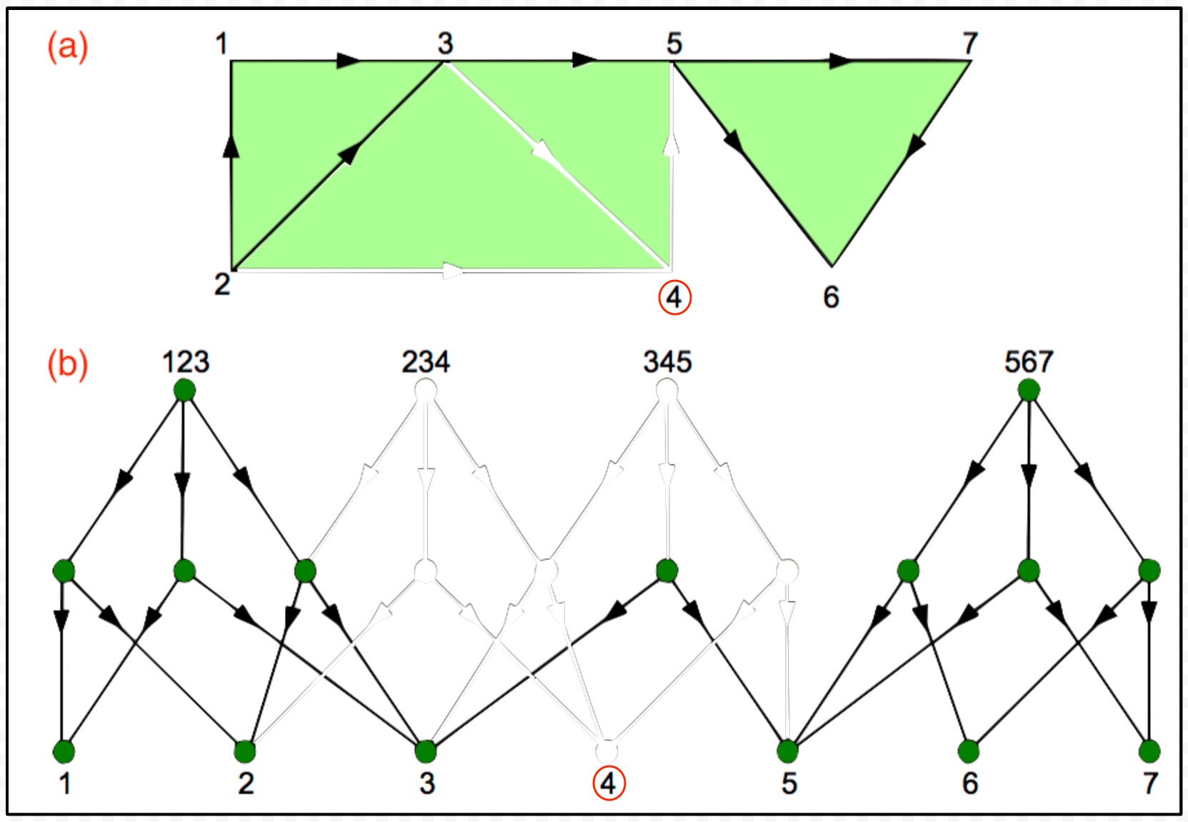Figure 2: In the above graphic, V is { 1, 2, 3, 4, 5, 6, 7 } and U is V − { 4 } = { 1, 2, 3, 5, 6, 7 }. The graphic shows (a) G_U the subgraph of G defined by restricting the set of vertices to U, and (b) the Hasse diagram H_U corresponding to G_U with the parts of H not included grayed out to illustrate the property of downward inclusiveness, i.e., the Hasse diagram of any subgraph of G is a subgraph of H.

For a region of size Width × Height × Depth and a particular Stride—assumed here for simplicity to be the same along all three axes—we will likely have a relatively large number of subregions and hence subgraphs for which we want to compute topological-invariant feature vectors⁶ Assuming we don't want to construct a new Hasse diagram for each H_U such that U ⊂ V and wish to parallelize the convolution algorithm by computing topological invariants for several subgraphs in parallel, there are a number of options that come to mind. In the following, we explore one such option that requires little modification of existing code and requires that we only compute H. With some abuse of notation, each vertex u ∈ U is a 0-simplex and hence also a vertex of H_U.

Actually, we don't have to explicitly construct H_U in order to compute feature vectors consisting of topological invariants; rather, we simply traverse the vertices of H that would have been present in H_U had we constructed it. Specifically, we modify computeHomology so that it can operate directly on H given a list U_start indicating which vertices of H to start at in order to (virtually) traverse H_U and another list of vertices U_stop indicating when to stop. In the following, H is simply treated as a directed acyclic graph—vertices corresponding to k-simplices with outgoing edges pointing to vertices corresponding to (k + 1)-simplices—with multiple roots corresponding to the vertices in V. U_start is just U ⊂ V. U_stop is obtained by performing a depth first search (DFS) of H starting from U with the following variation⁷:

Begin by setting U_stop to be the empty set { }. To distinguish from the elements u ∈ U from other elements of H not in U, we will use the variable v. The first time the DFS visits a vertex v, add v to U_stop, set n_v to 1 and then backtrack. We use n_v to keep track of the total number of times we've visited v during the DFS. Note that the in-degree d_v of a vertex v ∈ H is equal to 1 plus its depth d in H, and ∀ u ∈ U, d_u = 1. On each subsequent visit to a vertex v, increment n_v by 1. If n_v < d_v, then backtrack even if there are edges out of v. Otherwise, it must be that n_v = d_v, and therefore it follows that v ∈ H_U, and so remove v from U_stop and continue the DFS traversal if there are edges out of v. If v ∈ H_U the DFS is guaranteed to visit v exactly d_v times.

Now it should be relatively easy to modify computeHomology so as to implement a version computeLocalHomology such that computeLocalHomology(H, U_start, U_stop) = computeHomology(H_U). However, it would be almost as easy to simply overload computeHomology so that computeHomology(H) performs exactly as the original and computeHomology(H, U) directly incorporates the functionality described above for restricting attention to H_U which is guaranteed to be a subgraph of H.

May 25, 2016

Here's a brief report concerning the Neuromancer Rendezvous in Seattle this week: Breakfast at Google with Michael Buice to discuss the new datasets that we exchanged email on earlier in the week. (See here) for what I knew about these datasets prior to meeting with Michael.) Group meeting and lunch with Neuromancer and Clay's MindScope team along with Sebastian Seung's group at Princeton participating via video conferencing. I had additional meetings with Clay, Jerome Lecoq and Steven Smith later in the afternoon.

Clay told me that it would 2-3 years before we have aligned functional (calcium) and structural (connectomic) data and then only on mm³ samples. He said that in the meantime it might make sense to segment the rest of Wei-Chung's data [149] as "it is the best we'll have for years". Michael Buice—pronounced "bice" as in "vice" but according to Clay— had said that it might be some time before we have a Cre line for inhibitory neurons, but Clay said he expected to record from inhibitory neurons within couple of weeks and the dataset out within the next month and that a new Cre line wouldn't be necessary—they plan to use an existing Cre reporter line.

I saw Jerome Lecoq (<jeromel@alleninstitute.org>) in the meeting room next to ours and sent email suggesting we chat. He returned my message telling me to come by his lab to see his microscopes and experimental apparatus. Jerome indicated that Clay's prediction regarding when we can expected aligned, same-animal combined functional and structural datasets is consistent with his estimates. He opined that they would have multi-layer-location datasets somewhat sooner. Jerome was pessimistic about light-field scanning in deep tissue [156, 28], but suggested I take a look at work going on in Elizabeth Hillman's lab at Columbia.

Michael and I agreed that if we wanted to run the experiments I described to him anytime soon, our best bet might be to infer the connectomic structure from the functional data. I knew of some related work from Columbia University which I've queued up to read this weekend. The papers of Mishchenko, Paninski, Vogelstein and Wood [225, 178, 177, 176] are the only ones I found in my BibTeX database⁸ and their line of work appears to be the most cited work out there, but I expect there are some more recent ones I'm not aware of.

I also met with Steven Smith and we traded updates. I told him about how Neuromancer is progressing on fully-automated reconstruction and he told me about his recent array tomography work. At Paul Allen's urging, Steven has initiated an arrangement with a hospital in which he is supplied with mm³ — and larger — samples of human neural tissue that have been removed during surgery on patients suffering from a neurological disorder that ostensibly involves a portion of hippocampus adjoining the neocortex. According to Steven, Paul doesn't want his legacy "to be all about rodents."

Steven explained that rodent brain tissue is hard to work with in culture because it degrades quickly, allowing for at most a few of hours of in vitro recording and generally much less. Moreover rodent neurons rapidly generate new connections thereby masking the original circuitry. Steve explained that human neurons—perhaps because of their longer human life spans—are more stable and can kept alive and perform much as they would in an intact brain for many hours, even days. I read elsewhere that human cells in culture generated from induced pluripotent stem cells generally survive longer when densely populated, e.g., 50-100K cells, and survive even longer in tissue samples—corresponding to biopsies removed from patients during exploratory surgery—that include supporting structural proteins and glia.

Steven invited me to "high tea" which is a ritual performed each day on the sixth floor at 4pm and includes small, butter-rich English tea biscuits that Steven has obviously developed a taste for. Then I sent a note to Eric Jonas, Amy Christensen, and Vyas Saurabh asking for references on inferring structure from function, wrote this trip report in the executive dining room on the sixth floor overlooking Lake Union and walked back to the Ballard Hotel.

Miscellaneous loose ends: Read more carefully Jonas and Kording [126] and think about why Konrad might be far to pessimistic about the prospects for rich hierarchical models. Describe how the multi-scale, convolutional persistent homology can be applied to segment a connectome into functional parts and how those parts can be modeled with the dynamical systems methods that Semon, Wisam and Iran are working on for their projects.

May 23, 2016

Miscellaneous loose ends: Last week, an MIT student in Ed Boyden's lab asked if I had heard of "symbolic dynamics" and I drew a blank. As it turns out, however, I actually know quite a bit about the study of symbolic dynamical systems. [I couldn't quite say to him, "I've forgotten more about dynamical systems modeling than you'll ever know", but the part about "forgetting" was accurate enough.] At Brown University, starting in the 1995 Fall semester, I started teaching a graduate course on dynamical systems. The website still exists and comes up when you search for "dynamical", and "systems", but the material and level of mathematical sophistication is hopelessly outdated, and the field has advanced in some cases and been retarded by the influence of special-interest groups pushing particular modeling methodologies in other cases.

In the 1990's I spent several months at the Santa Fe Institute in New Mexico working with, among others, Jim Crutchfield who was one of the SFI / Berkeley/ UCSC "chaos" crowd, along with Farmer, Packard and Shaw [192, 70] who had just taken a "sabbatical" from SFI to try their hand at predicting financial markets [ostensibly to make lots of money for a major Swiss bank]. I drew inspiration for the course at Brown from an SFI monograph edited by Andreas Weigend and Neil Gershenfeld [267] and in particular work by Neil and Andreas as well as other scientists and mathematicians who contributed to their jointly edited collection of papers on time-series prediction [79, 216].

It was Jim's work that got me interested in state-space splitting and merging. Some of the motivations for studying such systems—see the preface to An Introduction to Symbolic Dynamics and Coding by Douglas Lind and Brian Marcus—has spurred work in other disciplines. For example, work by Michael Jordan, David Blei and Eric Sudderth and their students has resulted in much more rigorous methods for inferring stochastic processes—see for example Eric's paper "Split-Merge Monte Carlo Methods for Nonparametric Models of Sequential Data" (PDF). Mike's, David's and Eric's modeling work involving Dirichlet and Pitman-Yor processes has helped to transform—and make mathematically well grounded—multiple areas of research, including scene recognition in computer vision and document categorization in web search, that rely on inferring the arity of a discrete hidden variable such as the number of classes in a classification problem or the number of states in a dynamical systems model.

At one time, I spent considerable effort trying to apply the techniques described in a series of papers on "Bayesian Model Merging in Markov Models" by Andreas Stolcke and his colleagues at Berkeley [245, 244], before going back and learning more about simpler approaches from traditional time-series analysis [44, 255], stochastic automata theory [132, 111], optimal control [11, 88, 19], and traditional non-linear dynamical systems theory [247, 255]. My point, if indeed there is one, is that most of what you'll find within the narrow confines of what constitutes the purview of "symbolic dynamics / symbolic dynamical systems" — by which I mean the conferences, academic departments and journals that researchers who self-proclaim allegiance to this area of inquiry typically participate in — you will also find in more conventional fields of mathematics and automata theory.

And so, for what it's worth, my advice is to beware of the outliers; often, but obviously not always, they are outliers for good reason. It is also worth pointing out that many of the really disruptive, paradigm-shifting theories that turn out to be confirmed by experiment—usually after a considerable lapse in time due in large part to the chilly or outright hostile reception they receive from the incumbent owners of the theories about to be overturned, are also outliers, albeit a very small fraction of all outliers. And, if you want an introduction to how these ideas are applied with respect to neurons and neural circuits, you could do worse by consulting one or two of these: [36, 37, 246, 121, 144, 103].

A Stanford student wrote asking me about Benjamin Libet's experiments indicating that conscious intention to act appears, at least in some cases, to follow the onset of activity in the cerebral cortex—the so-called readiness potential—usually associated with commiting to act and what these experiments might imply about free will. I think there is no question that many of our routine activities are carried out with little or no conscious intervention. That neither bothers me nor does it necessarily imply that we have no free will. Let me explain what I mean from the perspective of a computer scientist.

Suppose we take some action without being aware we played any role in deciding whether or not to take that action. We can, however, accurately recall that we took the action and the circumstances under which it was taken. Now imagine that at some later time, with full conscious awareness, we ask ourselves whether it was the right action to take and conclude that some alternative action would have been more appropriate. We then associate the alternatve action with the original triggering circumstances, conditioning ourselves to take the alternative when circumstances present, just as Pavlov conditioned his dog to salivate whenever he rang a bell. The next time the triggering circumstances present, you automatically choose the more appropriate action selected earlier with no conscious deliberation on your part, nevertheless I warrant that you exercised free will in this case⁹.

May 21, 2016

My niece and nephew once removed¹⁰ were in San Francisco last week and so we met for dinner on Friday to catch up on news from our respective branches of the family. I had other meetings in the city and spent the afternoon at the Google office on Spear Street near the Ferry Building. With the hoards of developers flocking to MTV for the 10th Google I/O, it made a lot of sense to be elsewhere for the day. I borrowed the desk that Jon Shlens usually occupies when he's squatting in the SF office and I was pleasantly distracted by the spectacular view set directly in front of me:

At dinner we talked of many things but I was particularly struck by some comments my nephew made concerning his interest in finding therapies for neurological disorders thought to be caused or exacerbated by problems involving microglia. I had mentioned earlier that focused ultrasound¹¹ had shown some benefit in removing plaque in mice models of Alzheimer's disease and that one measure of success was that this intervention did not increase the number of active microglia which would have indicated a possible — overcompensating and potentially dangerous — immune response [150].

In my email thanking the two of them for a pleasant dinner and stimulating conversation, I asked my nephew to tell me more about the different roles microglia play in the central nervous system and his scientific interests in particular. Here's what he wrote in return:

DGM: Here is a lengthy recording of an all day conference put on a couple years ago by the National Institute of Alcohol Abuse and Alcoholism — on the role neuro-immune mechanisms play in addictive behavior and pathology. I found all of the talks fascinating, but the two to focus on regarding the role microglia¹² play in synaptic plasticity (both synaptic pruning and formation) and learning are by Wen-Biao Gan at NYU and Staci Bilbo at Duke. Gan's talk includes the two photon microscopy video of microglia in action — both under normal basal conditions and under conditions where a laser was used to lesion a small portion of the brain. [The full conference can be viewed here and the presentations by Gan and Bilbo are here if you don't want to watch the entire five hour video.]

After seeing how mobile microglia are (even under non-pathological conditions) he and colleagues set out to answer the question, why do these cells move around so much. And what they showed was that microglia were not only implicated in ongoing and regular synaptic pruning (which one might expect from a phagocytic immune cell) but they were also necessary to synaptic formation. So, they are critical players in the sculpting of the neural network not only in prenatal development when microglia first colonize the developing brain (after the developmental period when the neuronal population is already established, but before synaptic connections are formed, and/or awakened), but they continue to reshape the network through life as the brain learns and unlearns.

TLD: This is really interesting. As you probably know, filopodia are thin, actin-rich plasma-membrane protrusions that "function as antennae for cells to probe their environment" and play an important role in creating and extending dendritic spines in neurons. The creation of these extensions requires the assembly of cytoskeletal polymers from simpler monomers and their subsequent disassembly and recycling when the filopodia are withdrawn, all of which happens on a scale of a few seconds, minutes or days depending on the circumstances. My first hypothesis as to the function being served by the frenetic microglial activity featured in Wen-Biao Gan's presentation is that the microglia are garbage collecting the detritus left over following the withdrawal and disassembly of the filopodia. If this cellular house cleaning is not carried out efficiently, the extracellular space would soon be littered with garbage slowing the diffusion of neural-signaling and metabolic-processing molecules and thereby compromising normal cognitive function. The footnote at the end of this paragraph includes some research notes I made in developing a proposal for a possible project at Google that never got enough traction with management to see the light of day¹³.

DGM: Bilbo's talk is fascinating. And it was through her written work [22, 271, 21] — see here and here for recommended readings — that I first became interested in microglia and the brain's auto-immune and inflammatory response mechanisms and their possible relevance to CNS pathologies — including developmental network disorders such as autism, and schizophrenia, and neuro-degenerative disorders such as Alzheimers, MS and ALS. The project I am spending all of my time on now is an early stage pharma effort to develop a modulator of microglial activity which could be useful in the treatment of CNS disease or injury.

What Bilbo has shown is that if the brain of a rodent is exposed to some sort of immune challenge — or if the mother is — during the developmental window when microglia are helping first to construct the synaptic connections between neurons, those microglia are permanently altered (for life) such that they will over-respond with a destructive vengeance to a subsequent shock later in life leading to potentially debilitating neurological disorder such as, for example, schizophrenia. This was really, really exciting for me, in part because it suggests their may be a therapeutic opportunity to prophylactically inhibit microglial over-reactivity and protect the brain, but also that network disorders may be a function not of the 100 billion neurons themselves (which for the most part do not reproduce themselves), but of the 100 trillion synaptic connections between neurons which are very plastic while they exist and are also transient (they form and are pruned in the face of learning).

TLD: This does sound pretty promising. From my relatively naïve understanding of the relevant pharmacology and gene-based therapies, an over-response requiring a chemical-suppressor or the quieting of a genomic pathway would seem easier to manage than if microglia were not being activated at all [59]. [I'm getting ahead of myself. I just watched the video of Wen-Biao's presentation at the conference you mentioned and looked at his paper in Cell describing the study that the results he presents are based on [197]. Some things became simpler and others more complex. The tradeoffs are clearly complicated but at least I now understand your comment about cytokines.]

Bilbo's approach to unraveling the role of microglia was distinctively different from Gan's as her analysis relied on gene expression levels and genetic pathways, while Gan relied primarily on two-photon microscopy, Cre-mediated recombinant methods and pharmacological intervention with toxins such as tamoxifen. She did an excellent job demonstrating the power of these techniques for analyzing genetic pathways in understanding the role of chemokines and cytokines in particular. The take-away messages were clearly stated at the end of her talk, namely that (a) the behavior she observed did not appear to be an inflammatory response in the brain, but rather a neuro-immune signalling response, and (b) the immune molecules featured in her work are powerful modulators of plasticity and should be considered in the context of addiction.

DGM: I've lots of other references to microglia and the role of neuro-immune signalling (via cytokines like IL-1, IL-6, IL-10 and TNF alpha, BDNF...) and could send those along if any of this looks to be useful/interesting to you. I'll be really interested to hear what you think about it in terms of your work on machine learning, and how this kind of amazing network plasticity at the root of human learning might prove to be inspirational for modeling machines that learn. [I'm not sure how knowing more about microglia will help in building better learning algorithm. It certainly could, but given the technology used in Gan's lab and how long it took them to generate the data for the results presented in [197], I'm not sanguine that we'll receive enlightenment anytime soon. In any case, I find the potential therapeutic impact worth a closer look. Perhaps someone from my class will have some ideas and want to look deeper.]

Miscellaneous loose ends: In looking at how microglia impact addiction, neurodegenerative disease and disorders like autism, I was reminded of our confusion about the origin of chocolate and cocaine. I did a quick search and here's what I found out: (a) Chocolate is made from the fruit of the Cacao tree, Theobroma cacoa in the plant family Sterculiaceae. (b) Cocaine is made from the leaves of the Coca tree, Erythroxylon coca in the plant family Erythroxylaceae. (c) Cocaine has no connection with poppies; opium and heroin are the most common products of poppies.

May 19, 2016

Here are some excerpts from a conversation with Robert Burton [35] concerning the confusion about consciousness in academic—and in particular philosophical—circles versus the relative clarity we find in functional analogs of consciousness in control theory and cybernetics.

TLD: Jo and I just finished the Robert Wright interview with Aron Thompson, the philosopher from UBC. We have been listening to meal-sized installments when we have breakfast or lunch together. I was impressed with Aron's comment at the beginning of the interview noting that consciousness is a process, thinking he had the same thing in mind as I have, namely, a computational process, but now I'm not so sure. I think he missed a chance to make clear what Buddhists mean by awareness and out-of-body experiences, as well as pin down the notion of consciousness while keeping the spectre of dualism at bay. Basically consciousness is to a human what photosynthesis is to a plant, at least insofar as are both are processes central to the organism.
The digital computer also offers an explanation / justification for what Wright refers to as the "gaps between the phases of consciousness" or "the blinking view of consciousness" and Thompson is referring to when he mentions that there is "data from perceptual neuroscience that indicates what looks like a continuous field of visual awareness is actually made up of 'pulses' that are discontinuous and have to do with ongoing brain rhythms and that parse or frame stimuli into meaningful units."

Despite the confusion in how non-computer scientists and even some computer savvy experts talk about digital computers, they are actually implemented as analog circuits with a clock that orchestrates read and writes and initiates operations on operands stored in memory registers. The transistors and other components etched on the processor chip are analog devices and require time to transition from one state, say "on", to another, say "off" in the case of a simple binary latch used to implement registers, during which the information state of the latch is neither "on" or "off", and hence it is risky to apply an operator to operands stored in registers until the stored values stabilize.

RAB: When I was a resident in the 60's, it was widely held that the continuous stream of consciousness that we experience was nothing more than frames of experience welded together so seamlessly that they created what seemed like a steady flow of time and events. The oft-quoted prime example was flicker fusion rate—where individual visual experiences flowed at a speed sufficient to create the illusion of a continuous present, including the orderly flow of time (like the frame rate of motion pictures).

Even so, we can't viscerally understand how neurons create love and grief, and so we look to metaphors (man's way of explaining to himself what he cannot understand via equations and evidence). And we end up with the very cogent metaphor, photosynthesis is to plants as consciousness is to animals. Unfortunately, computer metaphor isn't emotionally satisfying to most people. (Reasons vary from not understanding how computers work to an ongoing sense that we wouldn't be unique or different from robots if all we are is computations).

Perhaps a useful analogy: Even if we understand gravity to be a function of the basic fabric of space-time, we think of gravity as a force. We cannot strip ourselves of the notion of gravity as the "attraction between two bodies." So the metaphor of "the force of gravity" works at the level of daily experience even when it isn't an accurate representation of the way gravity "works" or what it "is." Consciousness will continue as a puzzle even if it is fully understood at the physical level (just like gravity). People will continue to offer pet theories just as quantum physicists continue to root for the discovery of gravitons). It is our nature. Plants photosynthesize and we speculate.

TLD: And so perhaps I shouldn't disabuse others of their common-sense metaphors, especially, say, if they are comfortable with Newton's laws and never had cause to apply them to anything other than Newtonian circumstances that arise in daily life. However, there are cases when a more powerful metaphor helps as, say, in the case of gravitational lensing as means of constructing more powerful telescopes. In the case H. Sapiens 1.0, we are controlled to a significant degree in our social interactions by instincts honed by natural selection for a hostile environment we no longer inhabit. Luckily for us, civilization can effectively speedup natural selection.

Perhaps, if you had a better idea of what was happening in your brain, you might be able to redirect, harness or at least recognize when you are being ridden by instincts that are leading to bad outcomes. Or, if you aren't interested in why we behave as we do and can accept advice even when the reasons given are spurious, then you can still derive benefit by, say, miming a happy face, rearranging your body in a confident posture, wrapping your hands around a warm mug of tea, or speaking more slowly, distinctly and at a normal volume — all of which have been found empirically to improve mood, and for which we have some understanding of the relevant neural circuits, genetic pathways, neuromodulators, etc.

If we had a user's manual for H. Sapiens 1.0, it would surely include the following advice: losses compel more than gains, beware of the gambler's fallacy, power corrupts ... induces a sense of entitlement even in the best of us, social beings lie to themselves so they won't reveal their duplicity, and many others for which we have good evidence, and, in all the cases given here, some reasonable hypotheses about their neural correlates. There is a difference between using a metaphor as a heuristic or mnemonic for solving problems and believing the metaphor literally and having that belief bleed over into aspects of life for which it is completely inappropriate.

I think I'm being annoyingly pedantic and preaching to the choir. I get what you're saying. We all tell stories to supplement our understanding of complex systems; some believe those stories and take solace in their comforting familiarity more literally than others. None of us is far from the animal in the jungle, alert to every sound and movement, prepared to respond at a moments notice to whatever threat we encounter as our lives depend on it. "Faith in the unity of nature should not make us forget that the realm of life is at the same time rigidly unified abstractly and immensely diversified phenomenologically" ... Erwin Chargaff in warning his fellow molecular biologists not to become overly attached to their — increasingly abstract — theories or overly aggressive in selling their scientifically-motivated perspectives on life to the general public.

RAB: Ahh! Now we seem to be on the same page.

TLD: [Wool gathering] Think of a robot operating system (ROS) in which there is one master process called the controller, which has many sub processes that can run in parallel threads, one in particular we refer, to tongue in cheek, as the decider¹⁵ and will think of in the present context as the computational locus of the conscious self.

The remaining sub processes we'll refer to as the workers—though "worriers" might be more appropriate term—and they have access to a wide range of signals originating from the robot hardware, e.g., sensors and effectors, as well as from other workers. We treat consciousness as we would any other subprocess not because it's indistinguishable in either its specific activities or its neural substrate, but rather because it represents just another thread of computation that depends on an allocation of computing resources, can be sped up or slowed down by the operating-system process-scheduler, and can be put to sleep like any other process thereby curtailing its use of any resources until reawakened by the scheduler or a system interrupt.

News flash! Hold the presses. This story just in. — I was not looking forward to fleshing out the above narrative. Not because it would be particularly hard, but, rather, because it would be tedious and somewhat pointless. I'm not interested in explaining consciousness so as to account for the quirks of the human variant of consciousness. I'm an engineer and my only interest in consciousness now that I understand what it's good for and what purpose it can perform from a control systems perspective, is to construct particular instantiations of my systems-level understanding of consciousness useful for solving particular control problems. Well, that and because I'm a clever boy and believe that I could explain consciousness so a control theorist would recognize it immediately.

In any case, now I don't have to. Michael Graziano a psychologist and cognitive neuroscientist at Princeton has done it for me. Well, not for me in particular, and it needs some explaining, but Graziano has described a theory of consciousness that accounts for my systems-level understanding of consciousness and articulates it more clearly and comprehensively than I ever could or would have patience to do. Apparently he has written a book on the subject [94], but you can read his series of articles—linked to the publications page on his lab website at Princeton—in The Atlantic if you're interested [96, 97, 99, 95, 98].

I can only vouch for the articles in the January and June issues and recommend them highly. I'm so jazzed! It's like I had an assignment from my 5th grade teacher to explain the representatoin of self, attachment, transference, the difference between sensation, feeling and emotion¹⁶, etc. to a lay person and at the very last minute before school let out on a Friday afternoon she—her name was Mrs. Fisher and she taught me how to write good prose— decided to let us off the hook. Enjoy!

I'm re-reading selected excerpts of Horace Freeland Judson's The Eighth Day of Creation and reflecting on the character of the central players in this extraordinary of epoch of science, including Sydney Brenner, Francis Crick, Seymour Benzer and Fred Sanger ¹⁷. I expect I'm selecting on the basis of my preferences in personality since not all of the players in Judson's account were people I would like to have a relaxed dinner with to discuss life, work and science.

May 17, 2016

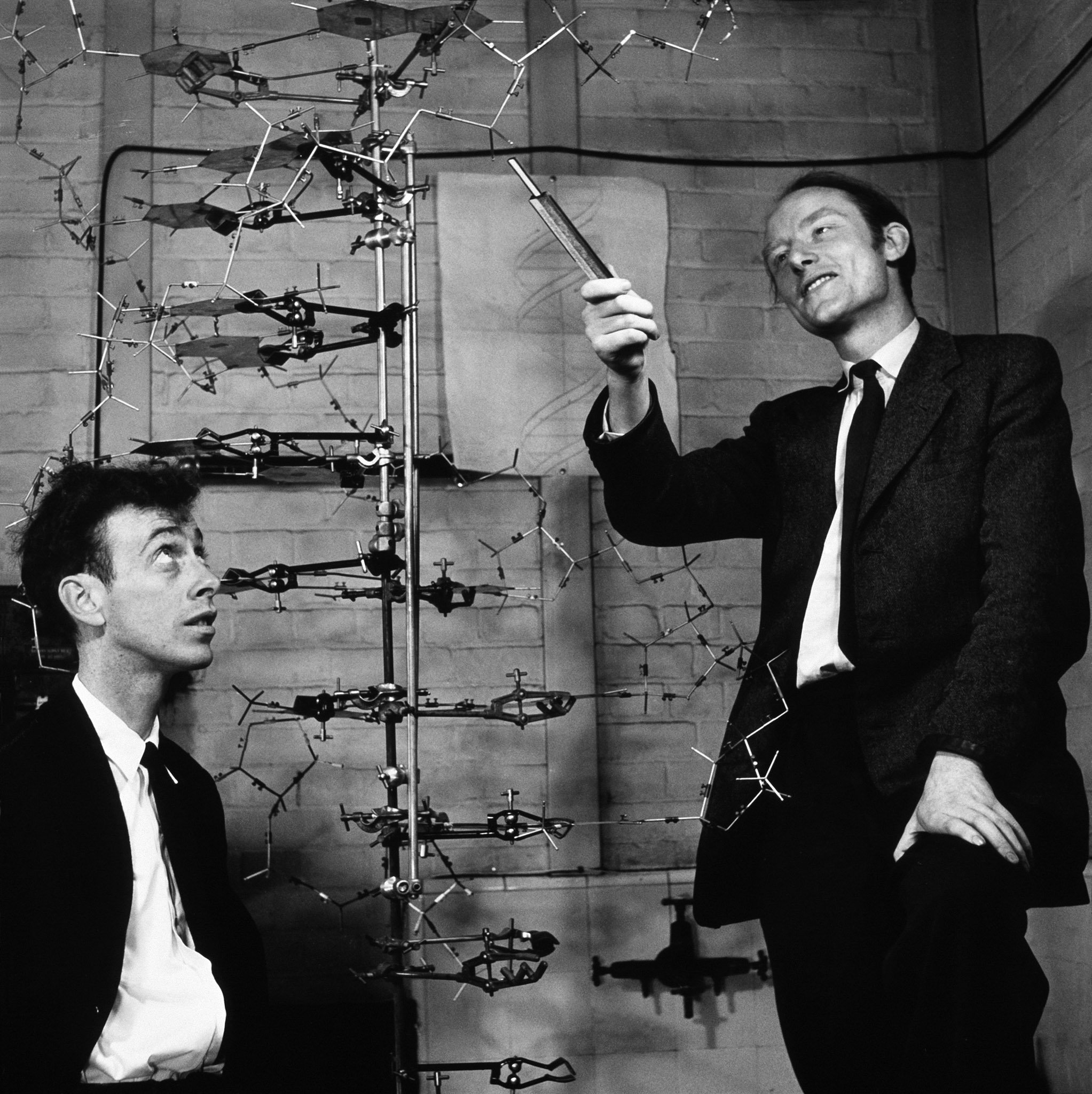
Wei-Chung ended his presentation with that famous (staged) picture of Crick and Watson standing next to a large model of the double helix with Crick pointing at the model with a slide rule and Watson looking on a little dumbfounded—see below. Wei-Chung made the point that having defined the structure of the genetic code, scientists had a model on which to fashion a functional account. It's worth pointing out that we're still just starting to make headway on this problem nearly sixty years after Crick and Watson's discovery.

The analogy to structural connectomics was obvious. Horace Freeland Judson's book The Eighth Day of Creation — which is, by all accounts, a popular science book of the first rank, written for a general but scientifically-literate audience, and revered by scientists — provides some hints about what might transpire as neuroscience tries to build a functional theory of neural computation on the structural backbone of the connectome [127]. The analogy has potential shortcomings.

In particular, there is no direct analog for the gene in the connectomic account, since the genome provides a complete account of both the structure and function of the organism; it's as though we knew about about the double-helix structure of DNA but hadn't a clue about how the nucleotide bases coded for protein. Of course, Jacques Monod and others have remarked, large proteins can fold in myriad ways and by so doing implement realize very different molecular machines, so maybe the analogy is more apt than it appears at first blush.

May 15, 2016

There have been some promising recent developments in the quest to build ultra-low-field MEG (magneto-encephalography) devices operating at room-temperature—no need for liquid helium cooling, providing a less expensive, less-cumbersome alternative to current SQUID-based (superconducting quantum interference) devices—no need for a room-size subject-and-sensor-enclosing Faraday cage, and relying on a tiny sensor compared to SQUID—some experimental devices are as small as 5 mm³ allowing for the possibility of monitoring brain activity in the case of unencumbered humans behaving in natural environments [81, 194, 214] — see this article on a device developed at NIST.

Unlike fMRI and SPECT, MEG is a direct measure—electromagnetic fields produced by current flow—of neural function. If it was simpler to use and less costly to purchase it would likely replace SPECT—which relies on injecting the patient with a radioisotope as a source of gamma-rays for imaging—for diagnosing neurodegenerative disorders. There are still S/N issues that need to be addressed in order to produce a reliable miniature sensor, but we believe these problems will be overcome in relatively short order given our current understanding of the relevant biophysics, and the improved spatial—on the order of a millimeter—and temporal—a millisecond or less—resolution coupled with the noninvasiveness of the procedure should create a demand for such instrumentation.

In January 2013, David Heckerman (UCLA and MSR) and I met in LA to discuss the practicality of using ultrasonic imaging to record activity in deep brain tissue. David did some work on this topic in his undergraduate thesis and I had been closely following the research of Lihong Wang on photoacoustic imaging with one of my former students who in an engineer working on ultrasonic imaging and stimulation at Siemens. In our 2013 technology roadmap we wrote that ultrasound imaging was beyond our five year planning window. But three years have passed and Lihong's work has exceeded our expectations to the extent that there may be reliable photoacoustic imaging devices within the next couple of years [277, 263, 72, 72, 138, 262] — see this NPR article featuring Professor Wang.

May 11, 2016

Summary: I. Change of venue for the class on Wednesday, May 26. II. New dataset soon to be released by the Allen Institute. III. Miscellaneous loose ends and class related updates.

I. Change of venue for Wednesday, May 26:

In class on Wednesday, we discussed the possibility of everyone car-pooling over to Google for the last class. Everyone present agreed this would be fun and so I'll arrange for it to happen. If you absolutely can't make it over to Google, I'll send you an invitation to the Hangout so you can participate virtually. This will be the last class of the course you will be expected to attend and so the meeting at Google will be a party of sorts replete with snacks from the MK (micro-kitchens) and perhaps some beer to lubricate your tongues and thus encourage questions and interactions. The last class features Peter Latham from the Gatsby Institute whom I visited recently and twisted his arm into giving a lecture. I'm also inviting several CS379C alumni including Amy, Mainak and Saurabh who've attended some of the lectures this year and several Google research scientists.

Directions: I'm in the 1875 Landings building at the corner of Landings Drive and Charleston—just Google 1875 Landings Dr, Mountain View, CA 94043 for directions. From Stanford, From Stanford, I usually drive straight down Embarcadero, across 101 overpass and then right on East Bayshore Road to avoid the traffic on 101. I'm expecting you to self organize to find transportation. If you don't have a car and can't find someone who is driving and has room, tell me and I'll help you arrange for transport.

II. New dataset released by AIBS in June:

Here is a recent email exchange with Michael Buice, a theoretical neuroscientist from the Allen Institute for Brain Science, concerning calcium imaging data acquired as part of Project MindScope [143] studying the mouse visual cortex:

TLD: Hi Michael, Costas said you were handling the CI data and would likely know what the status is. I'm developing a proposal for a functional modeling project to complement Neuromancer and part of that proposal will involve making commitments to milestones, etc. Clay told me that CI data would likely be available by the end of last summer or early fall of 2015, but if that happened nobody told us. Can you give me a status update? Thanks.
MB: Hi Tom, The Cortical Activity Map—that's our project name for the large-scale 2-photon data—just finished the first product run about 3 or 4 weeks ago. We're processing and packaging the data now and the first release will be in June with a following release in October, at which point you can freely download the data and APIs. If there's something you'd like to look at sooner than that, we might be able to arrange something. It would also be relatively simple to get you some example data sets.

This data set consists of recordings from roughly 20 "Locations", where a Location is defined as a tuple of (Cre line, region, depth). The Cre lines range over (Cux2, Rbp4, Rorb, Scnn1a), the regions over (V1, LM, AL, PM), and the depths over (175μm, 275μm, 375μm) (there's some variation in the exact depth of particular recordings). I've attached an image [included below] to help with this (ignore the dots for now, the shaded regions in that matrix correspond to Locations from which we've taken data). For each Location, there are 3 stimulus Sessions (where Session defines the types of stimulus used) that contain about an hour of recording from the same area of cells, with between 60-80% of cell ROIs matched across sessions.

The mice are active and engaged in passive viewing while being allowed to run. The set of stimuli across the 3 sessions are static and drifting gratings, locally sparse noise, natural scenes and movies, and spontaneous activity (grey screen). For each Session and Location, there are about 4 (a few have 8) experiments with different mice. In all, we have about 16,000 uniquely identified ROIs, roughly 10,000 of which have the complete set of stimuli. Let me know if you have any further questions and I'll assure you of a speedier response.

TLD: This is sounds like a super interesting dataset! Peter Li sent around this paper [169] to help us in sorting out the extra-striate regions that you mentioned. We were curious why you picked those regions? I don't know how the data was acquired, but, if the animals were allowed to run while viewing, will you also be able to provide behavior activity traces? Not sure how much influence this could have on activity in these visual areas, but it might be worth looking at if available.

Also — probably too much to hope for at this stage — is there an EM stack associated with this data? It would be very interesting to align the structural and functional data. I'd like to apply an analysis similar to the one described in [60] to such an aligned dataset. The students in my Stanford class this year are working on a bunch of projects investigating related issues. I'll be in Seattle for the Spring Neuromancer Rendezvous on May 26 and would love to get together and catch up.

There was follow up discussion organized by Jon Shlens a week later which is summarized in the footnote at the end of this sentence¹⁸.

III. Miscellaneous updates and references:

Video and audio for the Anastassiou and Boyden presentations are now linked to their calendar entries. Remember that Ed invited your questions following his presentation, if you had any but were too shy to ask during class:

May  9, Monday: Costas Anastassiou, Allen Institute for Brain Science (TALK) [RELATES TO SUGGESTED PROJECT #3]
May 11, Wednesday: Ed Boyden, Massachusetts Institute of Technology (TALK)
May 16, Monday: Wei-Chung Lee, Harvard University (TALK) [RELATES TO SUGGESTED PROJECT #2]
May 18, Wednesday: Adam Marblestone, Massachusetts Institute of Technology (TALK)
May 23, Monday: Project Discussions
May 25, Wednesday: Peter Latham, Gatsby Computational Neuroscience Unit (TALK) [TALK + END OF CLASS PARTY @ GOOGLE]

Here are some related references, including a chapter on micro-meso-macro models by Costas Anastassiou and Adam Shai appearing in a new compilation by György Buzsàki and Yves Christen (PDF), an interesting, but technically challenging paper suggested by James Thompson and another, suggested by Peter Li, that sorts out the different Cre lines in the AIBS calcium imaging datasets:

@incollection{AnastassiouandShai3MDB-16,
       author = {Costas A. Anastassiou and Adam S. Shai},
        title = {Psyche, Signals and Systems},
    booktitle = {Micro-, Meso- and Macro-Dynamics of the Brain},
       editor = {Buzs\`{a}ki, Gy\"{o}rgy and Christen, Yves},
    publisher = {Springer New York},
      address = {New York, NY},
         year = {2016},
        pages = {107-156},
}
@book{BuzsakiandChristen2016,
       author = {Buzs\`{a}ki, Gy\"{o}rgy and Christen, Yves},
        title = {Micro-, Meso- and Macro-Dynamics of the Brain},
    publisher = {Springer},
         year = 2016
}
@article{BuesingetalNETWORK-12,
       author = {Buesing, L.  and Macke, J. H.  and Sahani, M.},
        title = {Learning stable, regularised latent models of neural population dynamics},
      journal = {Network},
         year = {2012},
       volume = {23},
       number = {1-2},
        pages = {24-47},
     abstract = {Ongoing advances in experimental technique are making commonplace simultaneous recordings of the activity of tens to hundreds of cortical neurons at high temporal resolution. Latent population models, including Gaussian-process factor analysis and hidden linear dynamical system (LDS) models, have proven effective at capturing the statistical structure of such data sets. They can be estimated efficiently, yield useful visualisations of population activity, and are also integral building-blocks of decoding algorithms for brain-machine interfaces (BMI). One practical challenge, particularly to LDS models, is that when parameters are learned using realistic volumes of data the resulting models often fail to reflect the true temporal continuity of the dynamics; and indeed may describe a biologically-implausible unstable population dynamic that is, it may predict neural activity that grows without bound. We propose a method for learning LDS models based on expectation maximisation that constrains parameters to yield stable systems and at the same time promotes capture of temporal structure by appropriate regularisation. We show that when only little training data is available our method yields LDS parameter estimates which provide a substantially better statistical description of the data than alternatives, whilst guaranteeing stable dynamics. We demonstrate our methods using both synthetic data and extracellular multi-electrode recordings from motor cortex.}
}
@article{MarsheletalNEURON-11,
       author = {Marshel, James H. and Garrett, Marina E. and Nauhaus, Ian and Callaway, Edward M.},
        title = {Functional Specialization of Seven Mouse Visual Cortical Areas},
      journal = {Neuron},
    publisher = {Elsevier},
       volume = {72},
        issue = {6},
         year = {2011},
        pages = {1040-1054},
     abstract = {To establish the mouse as a genetically tractable model for high-order visual processing, we characterized fine-scale retinotopic organization of visual cortex and determined functional specialization of layer 2/3 neuronal populations in seven retinotopically identified areas. Each area contains a distinct visuotopic representation and encodes a unique combination of spatiotemporal features. Areas LM, AL, RL, and AM prefer up to three times faster temporal frequencies and significantly lower spatial frequencies than V1, while V1 and PM prefer high spatial and low temporal frequencies. LI prefers both high spatial and temporal frequencies. All extrastriate areas except LI increase orientation selectivity compared to V1, and three areas are significantly more direction selective (AL, RL, and AM). Specific combinations of spatiotemporal representations further distinguish areas. These results reveal that mouse higher visual areas are functionally distinct, and separate groups of areas may be specialized for motion-related versus pattern-related computations, perhaps forming pathways analogous to dorsal and ventral streams in other species.},
}

May 7, 2016

For those of you interested in macroscale networks inferred from MRI data using diffusion-weighted imaging techniques such as diffusion-tensor imaging (DTI), you might be interested in papers from the labs of Dani Bassett at the University of Pennsylvania and Xiao-Jin Wang at New York University. Both did their Ph.D. work in physics and both bring a refreshing-level of mathematical sophistication to their research. Matt Botvinick mentioned X-J Wang who is known for 'mesoscale' models of perceptual decision making. I ran across Bassett's TED talk and, despite it's TED-talk-audience-level of content, I found it intriguing enough to chase down her lab page and skim a few of her papers which are—as you might expect—considerably more contentful.

For relaxation this weekend, I read a general-audience science book [8] by a husband-and-wife team of research scientists at Stanford, Justin and Erica Sonnenburg, that discusses what we now know about how the microbial community, known as the microbiota, in the gastrointestinal tract or gut impacts our development, behavior, mood and immune system. Back in 2012, there were special issues of Nature and Science dedicated to papers about the microbiota of the gut. A year ago there was a much-read and talked-about article in the New York Times describing some of the research and quoting Tom Insel [4] concerning gut microbiota and related implications for health and human development¹⁹.

It is clear there is communication between the gastrointestinal tract and the brain when gut bacteria produce chemical byproducts that are absorbed through the wall of the small intestine, enter the blood stream, are carried to the brain and diffuse across the blood brain barrier to influence neurons and glia. We don't know the causal origin of the signal precipitating this cascade of activity nor do we know how, whether or to what extent feedback from brain is conveyed back to the gut bacteria. However, evidence is mounting that experimentally-induced changes in gut microbiota can influence immunological capacity, behavior and mood. The impact on development may be even more consequential for our long-term health, social flexibility and emotional well being.

In neuroscience, we are becoming increasingly aware of just how difficult it is to precisely modulate mood or behaviour by stimulating individual neurons or regions of the brain. In considering gastrointestinal interventions intended to modulate the size, diversity and spatial distribution of bacterial colonies in the gut, their precise control appears to be even more complicated to engineer. It's been known for decades [7] that bacteria form colonies, communicate with one another, coordinate to share scarce nutrients and even cooperate in repairing the compromised membranes of siblings by transiently fusing and exchanging their outer membrane contents [11]. There is also speculation that diversely-populated and structurally-organized super colonies—interconnected colonies of colonies—are capable of rudimentary information processing [11]. It remains to be seen just how complicated is the interplay between the gut, brain and immune system, but already it appears plausible that the gut plays a substantial role in regulating affect and may be implicated in a wide-array of mood disorders.

[1] Cao, X., et al. "Characteristics of the Gastrointestinal Microbiome in Children with Autism Spectrum Disorder: A Systematic Review." Shanghai Archives of Psychiatry 25(6):342-353, 2013.

[2] Goehler, L. E., et al. "Campylobacter Jejuni Infection Increases Anxiety-Like Behavior in the Holeboard: Possible Anatomical Substrates for Viscerosensory Modulation of Exploratory Behavior." Brain Behavior Immunology 22(3):354-366, 2008.

[3] Hsiao, E. Y., et al. "Microbiota Modulate Behavioral and Physiological Abnormalities Associated with Neurodevelopmental Disorders." Cell 155(7):1451-1463, 2013.

[4] Insel, Thomas. "The Top Ten Research Advances of 2012." National Institute of Mental Health Director's Blog, 2012.

[5] Lyte, M., et al. "Induction of Anxiety-Like Behavior in Mice During the Initial Stages of Infection with the Agent of Murine Colonic Hyperplasia Citrobacter Rodentium." Physiology Behavior 89(3):350-357, 2006.

[6] Messaoudi, M., et al. "Assessment of Psychotropic-Like Properties of a Probiotic Formulation (Lactobacillus Helveticus R0052 and Bifidobacterium Longum R0175) in Rats and Human Subjects." British Journal of Nutrition 105(5):755-764, 2011.

[7] Shapiro, J. A. "Thinking about bacterial populations as multicellular organisms." Annual Review Microbiology, 52:81-104, 1998.

[8] Sonnenburg, Justin and Sonnenburg, Erica. The Good Gut Taking Control of your Weight, Your Mood and Your Long Term Health. Penguin Press. 2015.

[9] Tillisch, K., et al. "Consumption of Fermented Milk Product with Probiotic Modulates Brain Activity." Gastroenterology 144(7):1394-1401, 2013.

[10] Vassallo, Christopher, Darshankumar T. Pathak, Pengbo Cao, David M. Zuckerman, Egbert Hoiczyk, and Daniel Wall. "Cell rejuvenation and social behaviors promoted by LPS exchange in myxobacteria." Proceedings of the National Academy of Sciences 112(22):2939-2946, 2015.

[11] Xavier, R. S., N. Omar, and L. N. de Castro. "Bacterial colony: Information processing and computational behavior." Proceedings of the World Congress on Nature and Biologically Inspired Computing, pages 439-443, 2011.

May 5, 2016

Here is an exchange with Rishi Bedi (RB) concerning their—Barak, Nishith and Rishi are collaborating as a team—project building on the work of Dlotko et al [60]. Rishi is responding to email from Pawel in which Pawl accepts our invitation to work together and try to replicate or extend the experiments in his paper either by providing us with the 42 microcircuits described in the paper or by our sharing the code with him so he can run the experiments himself on their microcircuits using machines at INRIA or ETH. In this exchange, I try to answer several questions posed by Barak, Nisthi and Rishi.

RB: Thanks so much for helping us with this. We have a few basic conceptual questions about the algorithm / what Tom proposed as a possible extension and wanted to run them by you — please excuse some of the questions which are definitely a result of our inexperience with topology.
The crux of what we talked about with Tom is computing topological features on local subgraphs instead of the entire graph. We're a little concerned this might lose out on important global properties (like large holes, the kind which seem the most informative) — do you think is a concern?

TLD: Of course, the local subgraphs lack a global perspective, and, of course, you'll lose information, but you will gain precision in your ability to characterize and compare smaller regions. Certainly, two vertices in a local subgraph may have a path between them that involves vertices not within restricted spatial extent of a given region of interest. Note this is true of almost any microcircuit we will work with in the near future since the microcircuit will necessarily correspond to a relatively small sample of tissue.

To motivate the computation of local characteristics, consider the following: When analyzing a photo, you often want to identify objects at different scales and relate them to other objects at the same or different scales. When viewing a city from a helicopter, the grid of city streets and alleys might look like a regular texture. When you look closer, the curtain wall of a lone building may fill your field of view and the arrangement of windows might appear as a pattern of similarly sized tiles. The people on the sidewalk will look like identical ants following scent trails, but when you zoom in further you can resolve individuals, the textures of their clothing, etc. Neural microcircuitry is similar — as would also be the case in looking at the micrograph of an Intel processor.

We fully expect the dominating circuit motifs to be different in different sub volumes at the same scale and as well as in separate sub volumes at different scales. However, we may find that if we define the right sort of hierarchy some of the same motifs appear at multiple scales / levels in our hierarchy; such graphs are said to be fractal or self-similar. Smaller volumes with characteristic circuit motifs are very likely to be the defining features of different layers in the six-layer, mammalian neocortex, and tools of the sort you are proposing to build could be used to search a large connectome for regions of other parts of the brain that exploit similar computational architectures.

It is also worth pointing out that we are not giving up on characterizing circuits of larger spatial extent. In particular, a multi-scale algorithm will subtend the entire microcircuit at its largest scale. As we learn more about neural circuitry, we will develop hierarchical representations in which the vertices at all but the lowest level in the hierarchy are themselves graphs in the next lower level in the hierarchy. For example, Hypergraphs, dendograms, and partially ordered sets represented as Hasse diagrams are all special cases of hierarchical graphs, as are the highway maps that Pawel described in his presentation.

RB: Does it make sense to apply our filter on regions of space segregated by Euclidean coordinates to achieve locality? If there's some neuron link between separate regions of space, do we just break them? Is this an open question we need to figure out, or is there an obvious answer we're missing, or is our segregation notion flawed?

TLD: As mentioned above, we are not so much "breaking" links or paths in the full graph, as restricting our attention to a subgraph defined by a particular spatial extent, i.e., a region of interest defined in terms of an embedding of the graph in a the 3D volume representing the original neuronal tissue. When thinking about the physical realization of a neural circuit, a 3D Euclidean space is a perfectly reasonable model. On the other hand, a complete graph of size k can be naturally thought of as a k dimensional surface characterized in terms of topological features such as holes and voids and higher-dimensional features.

RB: If the task is to parallelize the computation—and the spatial segregation described above makes sense, why is that not simply equivalent to excluding neurons that are outside the given filter area? For example, if we're computing the Betti numbers over the area enclosed by (a,b) and (c,d) (where c > a and d > b), why can't we just loop over everything connected to neurons that are within that range and exclude all neurons whose Euclidean coordinates fall outside it? It seems this would allow us to parallelize the computation of the filter over different areas without actually modifying the algorithm. Are we missing something about how the parallelism needs to work / what the data looks like / etc.?

TLD: You certainly could do that but it isn't necessarily the most efficient way to do so. Every spatially restricted local graph is a sub graph of the full graph. More importantly for our purposes, the Hasse diagram of for any spatially restricted local graph is a—downwardly-inclusive—restriction on the Hasse diagram for the full graph. This means that if we use Algorithm 1 [60] to construct the Hasse diagram for the full graph including all k-simplices up to k ≥ the number of vertices in the largest spatially restricted local graph we will encounter, then we can compute the Betti numbers and Euler characteristic for any subgraph directly from the whole-graph Hasse diagram without running Algorithm 1 again.

RB: How can you have a five-dimensional hole in a three-dimensional space? Are the neurons in fact embedded in a higher dimensional space, or are we misunderstanding what a Betti number of 5 implies?

TLD: The embedding of the microcircuit vertices in 3D Euclidean space has little to do with topology per se. Graphs are not geometric objects nor are they topological objects. A simplicial complex is an algebraic object—topological space—consisting of the union of points, line segments, triangles, and their n-dimensional counterparts (SOURCE).

May 3, 2016

This footnote²⁰ includes answers to the questions posed by students in response to Pawel Dlotko's video presentation last week.

May 1, 2016

There are neurons without dendrites and those without axons. When dendrites are present as part of a neuron, they can be found in one of two forms, which are apical and basal—also called basilar—dendrites. Apical dendrites can be divided into two categories: distal and proximal. In the case of pyramidal neurons in the cortex, the longer distal apical dendrites project from the cell body (soma) opposite from the axon. Distal apical dendrites form what are referred to as non-local synapses. Shorter proximal apical dendrites project radially to local pyramidal cells and interneurons. Pyramidal neurons segregate their inputs using proximal and apical dendrites.

Most neurons in the cortex have spines and so are called spiny neurons. The number of spines can range from around 10,000 on pyramidal and hippocampal neurons in the cerebral cortex to 100,000 on purkinje cells in the cerebellar cortex²¹. We often focus on the inner layer of cells in the cortex, but elsewhere in cortex we find interesting structure involving both novel forms of dendritic arbors and different types of neurons²².

Some of you remarked that you found it odd that Janelia places such an emphasis on the fly and zebrafish. In fact, the fly brain, while not including a neocortex, has many structures homologous to human structures and is particularly useful as a model in molecular and genetic neurobiology as one can raise many generations in a short time. For example, the fly olfactory bulb is an interesting part of the fly brain in part because it provides a good model for studying learning. The olfactory bulb is an ancient, highly preserved part of the brains of many organisms and exhibits some interesting dendritic and neuronal structures not found elsewhere in brains²³.

For example, the olfactory bulb in humans, mice and flies includes globular complexes called glomeruli that contain mitral cells that are enervated by many thousands of olfactory receptor neurons. The number of glomeruli in a human decreases with age; in humans that are over 80 they are nearly absent. The rapid reproduction cycle of the fly made it possible for Seymour Benzer to study the genes regulating simple behaviors and Edward Lewis to discover the bithorax complex and launch the field of developmental genetics, laying the foundation for our understanding of the homeobox (HOX) genes, that are highly conserved in all animals, and responsible for the development of basic body type.

Miscellaneous loose ends: Matt Botvinick sent me a good survey paper by Xiao-Jing Wang [266] entitled "Neural dynamics and circuit mechanisms of decision-making" that reviews work on mesoscale theories that account for decision making in humans.

April 29, 2016

On Wednesday, May 4, Steven Esser from Dharmendra Modha's lab at IBM Almaden will be visiting to talk about "convolutional networks for fast, energy-efficient neuromorphic computing". Feel free to invite your colleagues at Stanford who are interested in neuromorphic computing. On Steven's calendar entry I've included links to his recent paper [68] plus related work, including a paper on Neurogrid from Kwabena Boahen's lab [16].

If you're interested in a project on C. elegans relating to the presentations by Saul Kato and Andy Leifer, then show up for class on this coming Monday, May 2; the rest of you don't have to come to class, but you're welcome to come if you have questions concerning projects. In additional to the data from Andy's lab provided in the SI for his 2015 PNAS paper [185], we now have data from Manuel Zimmer's lab used in their 2015 paper [133]. The data is password protected; contact me if you want to use it in your class project.

If you're interested in a project relating to Eric Jonas talk on Monday, April 18 — topic #2 described here, tell me and I'll see whether it makes more sense to have you join us on Monday or schedule a separate time.

The class notes mention network motifs in several entries. These motifs are specific to—and defined in terms of—a given class of graphs, e.g., cellular or social networks, neural microcircuits, snapshots of the world-wide-web graph as it has evolved over time, etc. Since they are defined purely statistically, they may not have any significance from a functional perspective.

This Wikipedia page includes links to a dozen motif-finding algorithms as well a list of proposed or documented motifs along with their putative functions. There is also a short section on criticisms of motifs that might be worth looking at if you're skeptical of their value.

Remember that a draft version of your project proposal is due by midnight Monday, May 2 or whenever I get up (usually around 3AM), whichever comes first and the final version of your project proposal is due by midnight Monday, May 9. (Note that there was a typo in an earlier message where I typed "Wednesday, May 2" — there is no such date in 2016 — when I meant to type "Monday, May 2".)

Miscellaneous loose ends: Here are the slides and audio from Matt Kaufman's presentation in class this past Wednesday. Here's a new paper [116] in Nature on labeling fMRI data with semantics markers, and some related, visually-quite-cool neural eye candy from Jack Gallant's lab at Berkeley.

April 25, 2016

Alex Williams mentioned some interesting research in Michael Elowitz's lab at Caltech on using gene expression levels as a proxy for neural firing patterns. Note that this is not the same mechanism used in genetically encoded voltage indicator (GEVI) probes like Arclight — see Cao et al [41]. Alex has some ideas for a project attempting to better understand how measuring the gene-expression levels could be used to reconstruct the firing history of individual neurons noninvasively. Here's what he had to say:

There are a large number of genes that are expressed following increases in neural activity (c-Fos, Arc, NPAS4, many others). This expression is driven by second-messenger pathways, usually involving calcium (see, e.g., Richard Tsien's work). Recent work in systems biology (e.g. [Michael] Elowitz at Caltech) has shown that such pathways can be exquisitely sensitive to the pattern/frequency of activation, not just overall / average activity.
In the context of neurons, this means that different genes may be preferentially activated when the neuron bursts/fires at different frequencies. Thus, the expression of each gene is a filtered readout of the history of neural activity. If we know the activity-to-expression transfer function for each gene, then we can reconstruct an approximate firing history of the neuron, given measurements of gene expression. This is more-or-less analogous to taking measurements in the frequency domain and then reconstructing a signal in the time domain via inverse Fourier transform.

This could be useful as a experimental tool—i.e. a way to noninvasively measure activity across many many neurons ex vivo. There are good ways to estimate the expression levels of genes in single cells. Given this "snapshot" of gene expression, how well can we estimate / reconstruct the history of neural activity?

More interesting to me is that this could be used to understand many basic cellular process. A lot of these immediate-early genes are implicated in synaptic plasticity and memory. Neurons might be using this as a mechanism to read out their spiking history—I have ideas on this as well.

I propose modeling these possibilities as a way to point future experimental research in this promising direction. Unfortunately, there is little data to directly fit the activity-to-expression transfer functions (though the tools exist if we motivate the right people). I do have some ideas for using open access data from Buzaki to fit a basic first-order model.

Miscellaneous Loose Ends: Jonathan Wiener's book — Time, Love and Memory — about the life of Seymour Benzer and the early years of molecular biology had profound impact on my understanding of and approach to pursuing science [270]. I've referenced Wiener's book several times in these notes and highly recommend the book to any current or would-be scientist.

Just this past week I mentioned the use of bacteriophage in creating recombinant DNA and its application in genetically engineering organisms that express fluorescent proteins used in calcium imaging. Seymour Benzer invented some of the key technologies used in genetic engineering²⁴ and the method of transduction²⁵ was invented by Norton Zinder and Joshua Lederberg around the same time (1951) though another method called transfection²⁶ developed more recently (2012) is more commonly used today.

Good science writing like Wiener's Time, Love and Memory and his earlier, Pulitzer-Prize-winning account — The Beak of the Finch [269] — of how the nascent theory of natural selection made the transition from Darwin's original conjecture to a well-substantiated theory almost universally accepted by scientists, are, I would argue, an essential part of any scientist's education. You might put both these books in your backpack when you set out on whatever adventure you have planned for summer break.

Moving from science writing to science-fiction writing, research on functional connectomics will complement structurally-focused efforts and profit enormously from leveraging the knowledge gained in developing completely-automated segmentation algorithms and exploiting the availability of complete wiring diagrams for target tissue²⁷. If one thinks about how to reverse engineer a large-scale integrated circuit, structural efforts like Neuromancer²⁸ are focused on generating the wiring diagram, while functional efforts like Matrioshka²⁹ are focused on measuring, analyzing and abstracting neural activity: ... measuring activity ... think: inserting probes and measuring currents ... analyzing ... think: determining if a transistor is part of a pull-down circuit ... abstracting ... think: does this subnetwork implement a gate, a latch, or possibly a more complicated computational entity like a multiplexer or operational amplifier.

April 23, 2016

The audio for Andy's in-class discussion last Wednesday is available here. On the same page, you'll also find a link to the Nguyen et al [185] SI (Supplementary Information) PNAS site allowing you to download the data used in the paper, and a video with a condensed version of his talk in case you missed it or want to review the material. Andy mentioned to me that he had a larger set of raw data that he would be willing to share with students for class projects.

If you're interested, you should send Andy email (Andrew Leifer <leifer@princeton.edu>) and ask him about the raw data, copying me on the message. It's good for you to get used to contacting scientists, asking them questions about their work—most of the time research scientists welcome questions and love to talk about their work, and requesting access to data and related software—just how welcome these latter requests will be received depends a lot on the culture of the lab producing the data and how you engage the lead scientist who will expect you've done your homework.

It's about time you should be working on your project proposal. I made several suggestions for projects in class on April 6. Several of you have indicated interest in one or another of these, and those of you who haven't started thinking about projects, should start there. The calendar entry for this coming Monday, April 25 lists a talk by Pawel Dlotko. Pawel is in Poland and, given the time change and family obligations, he created a video presentation that you can find here. Class participation will work a little differently for Monday's class, so keep reading this note, as it may not be necessary for you to attend class on Monday:

All of you should read the paper, watch the video and send me one or more questions for Pawel concerning his talk and paper. Your questions should address the technical content of his research and should be clear and self-contained. I expect each of you to send me your question(s) by the end of class time on Monday, April 25.
If you're interested in working on a project related to Pawel's research or to the data from the Human Brain Project that he and his co-authors used in their experiments, show up for class on Monday (April 25) and we'll work on developing ideas for related projects and identifying options for acquiring experimental data.
If you're not interested in this topic but you are interested in a project relating to work on C. elegans presented by Saul Kato on Monday April 4 and Andrew Leifer on Wednesday, April 20, then you'll have the opportunity of participating in an in-class discussion about projects relating to C. elegans on Monday, May 2.
If you're interested in a project relating to Eric Jonas talk last Monday, April 18, or you've talked with me about an alternative topic for a project, you don't have to attend class April 25 or May 2, though you still have to send me a question about Dlotko's paper "postmarked" no later than the end of class time on Monday, April 25.

Everyone has to send me a rough draft of your project proposal by the end of day on Wednesday, May 2. This will give me time to provide feedback before you write the final proposal. The basic content and format for project proposals hasn't changed over the years and so you can check out the Proposal Components and Example Project Proposal sections of the 2013 project description page here for guidance—obviously the 2013 topics are not relevant to this year's course. I expect the final draft of your project proposal by end of the day on Monday, May 9.

Aside from the two in-class project discussions on May 25 and April 2, I expect you to attend all the remaining classes or tell me in advance that you are unable to for some reason. As pointed out earlier, I expect attendance and participation because (a) it's the most valuable component of the educational experience this class offers and (b) because the scientists who have agreed to take the time to prepare and present their work deserve an engaged, enthusiastic audience.

Andrew Leifer's talk was a great example of what you can expect from our speakers but it was only sparsely attended. Fortunately, Andy provided a short video summary, but the "unplugged" audio recording has a lot of great material not included in the video. Thanks in advance for your help in making this a great experience for participants and invited speakers alike.

April 21, 2016

At the beginning of his presentation in class yesterday, Andrew mentioned Princeton's five-year postgraduate fellowships that include generous support for labs and equipment plus funding for students and postdocs, and the ability to work on hard problems that may take multiple years to make significant progress on. Andy's work and that of the students in his lab has dramatically demonstrated how such financial and programmatic freedom can produce exciting new science. I'm mentioning it here, I start recording the audio of his presentation after he'd made a plug for the program. You can find out more about the Lewis-Sigler Institute for Integrative Genomics here and the Lewis-Sigler Fellowship Program here.

I think Andrew and probably some of researchers in his lab would love Jonathan Wieners's book Time, Love, Memory: A Great Biologist and His Quest for the Origins of Behavior. The book focuses on Seymour Benzer's research from the early days of molecular biology when he was using phages to study bacteria to his ground-breaking work on the behavior of flies. There is an interview with Benzer conducted by his protege at Caltech, David Anderson, on the Genetics Society of America Oral Histories website that nicely summarizes Benzer's contributions³⁰.

The title of Wiener's book refers to three important discoveries in molecular and behavioral genetics that Benzer was involved with: time — work with his student Ron Konopka isolating the "period" gene governing the fly sense of time, love — work with Michael Rosbash identifying the per protein and showing how "period" mutations alter circadian rhythm and have a crucial impact on the mating song of the male fly — an incredibly complex behavior, and memory — demonstrating that flies learn from experience using a very clever experimental design.

The interview with Edward Lewis describes Lewis' nearly fifty years of isolated research in his basement lab at Caltech during which he published very little. When he finally emerged with 50+ page journal article, he had solved one of fundamental problem in genetics, namely, how the bodies of flies and humans develop from germ cells to fully functional organisms. He received the Nobel Prize for his discovery of the bithorax complex (BX-C) in Drosophila Melanogaster that led to the identification of the homeobox and to the realization that Hox gene clusters like the BX-C control the specialization of body regions in most, perhaps all, animal forms.

That went on for much longer than I initially intended, but Andrew's story about finding the protein-sensor and associated pattern generator responsible for propagating a motion-inducing wave along the worm's length [268] reminded me of how long each of the above-mentioned three discoveries—time, love and memory—took from inception to the publication of the key finding.

And, while I'm dredging up anecdotes from the history of science, Andrew's modus operandi reminded me of engineer-scientists from the 17th century like Robert Hooke who built the most sophisticated microscope of his time and the book he published Micrographia and the work of Michael Faraday in the 19th century who built the first solenoid, transformer, generator and motor and was renowned in London for his skill at orchestrating public demonstrations—basically reproducing experiments he'd painstakingly refined for the public—for the Royal Society and being an extraordinary expositor of science.

In each case, having built a scientific instrument, they exploited their industry by performing the first experiments using it, often perfecting the instrument in the process. Fortunately for Andrew, engineer-scientists are acknowledged as essential to modern science and well rewarded both academically and monetarily, unlike their counterparts in earlier centuries when the high-born scientists of the age would not sully their hands with menial work and disparaged the work of the artificers whose instruments they depended on for their dilettantish pursuits—indeed the word "dilettante" didn't have the pejorative connotation normally associated with it nowadays.

I've tracked the technology for Ca⁺² imaging for several years now and seen some pretty amazing pieces or hardware coming out of Ed Boyden's, Mark Schnitzer's and Alispasha Vaziri's labs but I'm really impressed with the both the hardware and control software from Andrew's lab. The precision and quantity in tracking neurons, the fact that he can perform six full-brain-scan frames per second, with five or six layers per scan and his ability to both activate and inhibit multiple neurons with exquisite precision is really incredible.

Thanks to Andy for the pointer to Gordon Berman's research and his lab at Emory. The Journal of the Royal Society paper with Choi, Bialek and Shaevitz [18] that he mentioned in class is super interesting and should be on the reading list for any student considering a possible project involving C. elegans. For students in CS379C, both Berman et al [18] (ACCESS) and Wen et al [268] (ACCESS) are open-access and available by following the supplied links.

April 17, 2016

Here's an email exchange with Pawel Dlotko with my feedback on the first draft of the video presentation he put together for CS379C:

TLD: You did a nice job presenting the basic ideas. The slides are clear and well thought out, and the introductory material on algebraic topology was particularly well done. Given that you're working on persistence landscapes and knowledgeable about persistent homology, I was wondering if you saw applications for these tools in neurobiology.
PD: Yes, we use statistical methods for persistence, but not to this particular project. We use it to classification and detection of diseases based on some information form MRI scans of a brain. To be precise, we are working on scans of a brain of patients with and without schizophrenia. However the results are not as good as I wish for. We get the difference in persistence (by using permutation tests), but so far we were not able to turn it into a classifier. The classification is apparently possible by using other standard ML methods.

There is also a potential use of statistics for persistence in the Blue Brain project. In fact, there are some ways to define weights on the connections. But as far as I understand it is not very clear how do it, that is why we are not there yet. I have also a version of a code for weighted networks, but it is not yet available online. If you see a need for it, I can work on it in a quite near future.

TLD: I would have spent a little more time trying to connect the topological analyses to the neuroscience, but you know better than I do what your colleagues learned from the exercise and what they deemed most interesting. Hopefully you conveyed whatever insights they gained. By the way, here's how you pronounce the word motif.

PD: Sorry about that. If you want I can make another record, but due to a traveling and talks tomorrow and on Friday I will be only able to do it during the weekend.

TLD: What biology you did delve into in any depth, you did well on. For example, you did a good job on the point versus circle stimuli, but I would have covered the transmission-response paradigm in a little more detail prior to talking about the experiments, using Figure 4 to illustrate.

PD: As below, I can add this detail. There are two parts that comes into this: (a) the real definition of the activity subcomplex, and (b) how we pick the time delays. (a) is interesting, while (b) is quite technical.

TLD: It would also be interesting to hear what you would have done differently or in addition had you more time to devote to a more in-depth analysis. For example, can you imagine an alternative, more expressive / biologically relevant simplicial complex.

By the way, I found the last ten minutes of the video, in which you discuss the notion of (information) highway graphs, intriguing and thought provoking. I expect the students will find it so as well and have lots of questions regarding the ideas and their application in neuroscience.

PD: This is a great question [that] I've been asking myself. While I cannot speak [authoritatively] about biological relevance, I can give you some of my intuition that comes from dynamics. And there are at least a couple of ideas I would like to check, but did not yet get the data:

There is [the] immediate question: Is there any [neurophysiological] functional meaning [to] homology classes? My intuition [in this case] is the following: Imagine a 1-d (for the sake of argument) cycle that is not bounded. I am wondering if we [would observe] a wave of activation [propagating] around this cycle. And, of course, [there would be] similar phenomena for higher dimensional classes. I have some ideas [on how to check this] based on my work in electrical engineering, but have not [done so] yet. There are, of course, [technical problems involved in setting up such experiments, and that is why we have yet to perform them].

Another dynamical question I want to answer is the following: Let a space of n-dimensional highways (for your favorite n) be our base space. First of all, I would like to see how much do we lose if we restrict activity only to the neurons that [comprise] the highways. I would also like to decompose the dynamics of the highway graph into recurrent and gradient-like dynamics (which is almost exactly the decomposition of a directed graph into maximal-strongly-connected-path components (recurrent) and the connections between them (gradient-like)) and see if this decomposition has any functional meaning.

PD: If by any chance you have some data that can be used for this purpose, I will be happy to try it!

TLD: What sort of circuit motifs do you think the current analyses miss? What do think you'd observe if you were using a more complicated stimuli? What sort of response plot might you observe if you had data from real mouse barrel cortex?

PD: Yet another good questions. The fair answer is that I do not know and I would prefer not to speculate.

TLD: In any case, one can always ask for more; you did a good job over all and it will certainly suffice for our immediate goal of informing the class and spurring them to think about the applications of such modeling techniques.

PD: I will try to give it another try during the weekend. If I make it, I will let you know.

April 11, 2016

In an earlier entry in this log, we considered a convolutional version of Algorithm 1 in [60] that would allow us compute topological invariants including Betti numbers and Euler characteristics of local regions at multiple scales. The rationale was that, while computing invariants of a large neural circuit might give us a signature that could be compared with other large circuits, much of what we hope to learn concerning computation is likely realized in terms of smaller, local circuits. These smaller circuits might correspond to primitive computing units for performing a specific function that appear in locations scattered about the brain—think of a logic gate or operational amplifier—or aggregated together in groups—think of a memory register or full adder—or as comprising a cortical layer or other morphologically distinct feature—think of a gate array or crossbar switch. The earlier entry suggests some data structures for implementing such a convolutional filter, this log entry just adds to the story by graphically describing the embedded microcircuit graph.

The main result of Dlotko et al [60] consists of a topological analysis of the structural and functional connectivity of 42 reconstructed microcircuits generated from the model described in [166]. The structural connectivity of each reconstructed microcircuit can be represented as a directed graph with approximately 3 × 10⁴ vertices and 8 × 10⁶ edges, while its functional connectivity is represented as a time series of subgraphs—called transmission-response graphs—defined by the functionally-effective connections at different times in the simulated neural recordings. As pointed out in the earlier entry, we need only generate the Hasse diagram representing the directed-flag simplicial complex for the complete microcircuit used in the structural analysis, since the Hasse diagrams for the transmission-response-graph complexes used in the functional analysis are all subgraphs of Hasse diagram for the complete microcircuit. Figure 1 below describes how the spatial layout of the reconstructed neural tissue plays a role in the convolutional algorithm.

Figure 1: Given the directed graph G = (V, E) corresponding to a reconstructed microcircuit and a mapping φ from vertices to their 3D coordinates in the reconstructed (neural tissue) volume φ(V) → { ⟨ x_v, y_v, z_v⟩ | ∀ v ∈ V }, (a) shows the vertices embedded in the reconstructed volume along with the edges representing their (static) structural connections—the graphical realization of the edges of G as straight arcs obviously has no physiological significance apart from representing connectivity, (b) depicts the 2D projection of a convolutional sliding window with stride equal to the window width, and (c) emphasizes that the (dynamic) functional connectivity—highlighted here in red—is typically a proper subgraph of the (static) structural connectivity. While obvious to some, I hope this graphical aid will make most our earlier conversations clear.

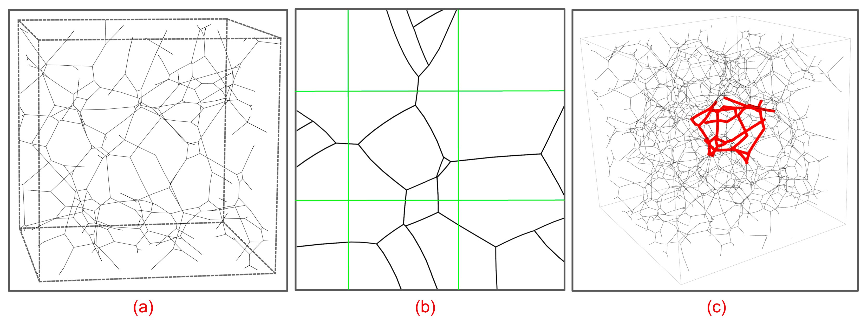April 9, 2016

Class Announcements:

Here are links to the papers for the lectures on Monday and Wednesday of next week, plus advance notice of the lecture on May 4 by Steven Esser from IBM Almaden on training deep networks by backpropagation using IBM's TrueNorth technology for anyone interested in neuromorphic computing especially students working in Kwabena Boahem's lab. The results described in Esser et al [68] using TrueNorth also bode well for Professor Kwabena's Neurogrid and the related technologies being developed in his lab.

Monday, April 11 — David Sussillo, Google Research
Wednesday, April 13 — Jeremy Freeman, HHMI Janelia Farm
Wednesday, May 4 — Steven Esser, IBM Almaden Research Center

Project Discussions:

For those of you caught up in the controversy concerning the scientific merits of connectomics, either because of your own dispositions or those of your academic advisers, you might want to consider the controversy that met Jim Watson's first public lecture on the helical structure of DNA at Cold Spring Harbor in 1953 or Seymour Benzer's³¹ first lectures in Roger Sperry's lab at Caltech on the advantages of studying fruit flies in order to understand the molecular basis of heredity. The heated controversy that erupted in Sperry's lab as a result Benzer's lectures was polarizing and the repercussions reverberated far beyond that one lab.

To put my cards on the table, I'm not at all conflicted about the importance of pursuing connectomics. I'm reasonably confident that we are going to learn an enormous amount about brains, biology, neuropathology and, ultimately, biological computation from studying the connectomes of diverse organisms. History has shown that this is not the sort of debate to be played on a large stage, not a war to be won by words, but rather a scientific question that will be resolved by scientists following their intuitions and honestly evaluating the work of their peers. I believe the next few years of research on functional and structural connectomices will settle the matter for most of those scientists whose minds are not already made up.

In class on Wednesday, I mentioned Saul Kato's comment concerning ensembles of correlated C. elegans neurons that feed into solitary neurons apparently—and this is just one possible hypothesis—serving as gating functions. Okun et al [188] showed that some neurons in a network exhibit spiking activity that is tightly correlated with the average activity of the population of neurons in the network—they christened these neurons choristers, while other neurons—christened soloists—display a diversity of spiking patterns whose correlation with that of the population is smaller than expected by chance, which suggests they actively avoid correlating with the rest of the population.

Here's a link to the EU Human Brain Project's Neocortical Microcircuit Collaboration (NMC) portal. The microcircuit connectomes analyzed in Dlotko et al [60] were generated from the cortical model featured on the NMC website and first described in Markram et al [166]. I'll ask Pawel Dlotko if we can use the models he and his coauthors used in their analyses. You can find Pawel Dlotko's C++ code for constructing directed-clique simplicial complexes and computing topological invariants here. Implementing a convolutional version of Pawel's algorithm to compute topological invariants of spatially localized subgraphs would make for a very interesting project.

Amy Christensen (chandra.christensen@gmail.com) and Saurabh Vyas (smvyas@stanford.edu) were in CS379C last year and used data from Costas Anastassiou's lab at the Allen Institute for Brain Science in their project. They did some additional work on the project over the summer and presented their findings at COSYNE last month. Amy and Saurabh offered to help out those of you interested in using Costas' data in your projects, and will make available the Python and Matlab scripts they developed to read the data and perform some basic preprocessing including the generation of adjacency matrices for synthetic cortical microcircuits.

Here is a relatively recent lecture by Andrew Leifer covering the material in his PNAS paper [185]: Whole-brain neural dynamics and behavior in freely moving nematodes. I've asked Andrew to tell us what published data he has that CS379C students can use in projects. I've also asked Saul Kato, but I'm pretty sure he got his data from Alipasha Viziri's lab [201]. I'll ask Alipasha if that's the case. An interesting and challenging project would be to see if you could automatically—or semi-automatically—infer an equivalent model from the original data used by Kato et al or the data acquired by Andrew's significantly improved imaging and tracking technology.

April 7, 2016

A couple of students have asked about the prospects for the field neuromorphic computing to have a practical impact in the next few years. There are a couple of prerequisites for that happening: First, we need real, working chips along with demonstrations that they deliver on the ultra-low-power promises often touted in the literature as being one of the primary reasons for pursuing this line of research. Second, we need examples of these chips implementing algorithms that carry out computations that we care about and that perform at or better than implementations running on traditional computing hardware, where by "perform" I mean in terms of speed and accuracy.

There are a number of recent published results worth mentioning: Kwabena Boahem, a student of Carver Meade, working at Stanford has a neuromorphic chip with an interesting solution to the interconnect problem that looks very promising [16]. Those of you who asked about neuromorphic computing were aware of Professor Boahem's progress and so I won't say more about his work, except to recommend that you visit his website and, if this area of research interests you, seriously consider taking one of his courses.

Dharmendra Modha and his team at IBM Almaden Research Center have been working on neuromorphic computing for some time now. Their 2009 paper [8] was somewhat controversial for its comparisons with biological brains, but their 2014 paper in Science provided a glimpse of what their chip—called TrueNorth—was potentially capable of [172]. The latest from Modha's group [68] has delivered on earlier promises by demonstrating how TrueNorth can train and perform inference on deep networks with very low power consumption and deliver state-of-the-art performance. In terms of power, right now the biggest benefits would come from very-long-battery-life portable devices, but obviously there are also reasons to pursue for applications in large data centers.

Below I've listed several recent, relevant citations from my bibtex database. The first author on the IBM paper, Steven Esser, will be participating in class on May 4, and, Greg Corrado, a student of Bill Newsome's whom I hired at Google some years back, worked at IBM on the DARPA SyNAPSE project that developed the TrueNorth chip and its software stack. I've also looked carefully at the memristive technologies that HP Labs and various semiconductor companies have been pursuing. HP's effort was the most publicized but apparently downsized when progress was slow delivering working machines. However, researchers have used memristive RAM chips from Rambus to do some interesting experiments. There are other players than those listed but these alone would justify pursuing this line of research for commercial applications. Here are the citations:

@article{EsseretalCoRR-16,
       author = {Steven K. Esser and Paul A. Merolla and John V. Arthur and Andrew S. Cassidy and Rathinakumar Appuswamy and Alexander Andreopoulos and David J. Berg and Jeffrey L. McKinstry and Timothy Melano and Davis R. Barch and Carmelo di Nolfo and Pallab Datta and Arnon Amir and Brian Taba and Myron D. Flickner and Dharmendra S. Modha},
        title = {Convolutional Networks for Fast, Energy-Efficient Neuromorphic Computing},
      journal = {CoRR},
       volume = {arXiv:1603.08270},
         year = {2016},
     abstract = {Deep networks are now able to achieve human-level performance on a broad spectrum of recognition tasks. Independently, neuromorphic computing has now demonstrated unprecedented energy-efficiency through a new chip architecture based on spiking neurons, low precision synapses, and a scalable communication network. Here, we demonstrate that neuromorphic computing, despite its novel architectural primitives, can implement deep convolution networks that (i) approach state-of-the-art classification accuracy across 8 standard datasets, encompassing vision and speech, (ii) perform inference while preserving the hardware's underlying energy-efficiency and high throughput, running on the aforementioned datasets at between 1100 and 2300 frames per second and using between 25 and 325 mW (effectively > 5000 frames / sec / W) and (iii) can be specified and trained using backpropagation with the same ease-of-use as contemporary deep learning. For the first time, the algorithmic power of deep learning can be merged with the efficiency of neuromorphic processors, bringing the promise of embedded, intelligent, brain-inspired computing one step closer.}
}
@article{BenjaminetalIEEE-14,
       author = {Benjamin, Ben Varkey and Gao, Peiran and McQuinn, Emmett and Choudhary, Swadesh and Chandrasekaran, Anand and Bussat, Jean-Marie and Alvarez-Icaza, Rodrigo and Arthur, John V. and Merolla, Paul and Boahen, Kwabena},
        title = {Neurogrid: A Mixed-Analog-Digital Multichip System for Large-Scale Neural Simulations},
      journal = {Proceedings of the {IEEE}},
       volume = 102,
       number = 5,
         year = 2014,
        pages = {699-716},
     abstract = {In this paper, we describe the design of Neurogrid, a neuromorphic system for simulating large-scale neural models in real time. Neuromorphic systems realize the function of biological neural systems by emulating their structure. Designers of such systems face three major design choices: (1) whether to emulate the four neural elementsVaxonal arbor, synapse, dendritic tree, and somaVwith dedicated or shared electronic circuits; (2) whether to implement these electronic circuits in an analog or digital manner; and (3) whether to interconnect arrays of these silicon neurons with a mesh or a tree network. The choices we made were: (1) we emulated all neural elements except the soma with shared electronic circuits; this choice maximized the number of synaptic connections; (2) we realized all electronic circuits except those for axonal arbors in an analog manner; this choice maximized energy efficiency; and (3) we interconnected neural arrays in a tree network; this choice maximized throughput. These three choices made it possible to simulate a million neurons with billions of synaptic connections in real time for the first time using 16 Neurocores integrated on a board that consumes three watts.},
}
@article{GokmenandVlasovCoRR-16,
       author = {Tayfun Gokmen and Yurii Vlasov},
        title = {Acceleration of Deep Neural Network Training with Resistive Cross-Point Devices},
      journal = {CoRR},
       volume = {arXiv:1603.07341},
         year = {2016},
     abstract = {In recent years, deep neural networks (DNN) have demonstrated significant business impact in large scale analysis and classification tasks such as speech recognition, visual object detection, pattern extraction, etc. Training of large DNNs, however, is universally considered as time consuming and computationally intensive task that demands datacenter-scale computational resources recruited for many days. Here we propose a concept of resistive processing unit (RPU) devices that can potentially accelerate DNN training by orders of magnitude while using much less power. The proposed RPU device can store and update the weight values locally thus minimizing data movement during training and allowing to fully exploit the locality and the parallelism of the training algorithm. We identify the RPU device and system specifications for implementation of an accelerator chip for DNN training in a realistic CMOS-compatible technology. For large DNNs with about 1 billion weights this massively parallel RPU architecture can achieve acceleration factors of 30,000X compared to state-of-the-art microprocessors while providing power efficiency of 84,000 GigaOps/s/W. Problems that currently require days of training on a datacenter-size cluster with thousands of machines can be addressed within hours on a single RPU accelerator. A system consisted of a cluster of RPU accelerators will be able to tackle Big Data problems with trillions of parameters that is impossible to address today like, for example, natural speech recognition and translation between all world languages, real-time analytics on large streams of business and scientific data, integration and analysis of multimodal sensory data flows from massive number of IoT (Internet of Things) sensors.}
}
@inproceedings{BojnordiandIpekHPCA-16,
    author = {M.N. Bojnordi and E. Ipek},
     title = {Memristive Boltzmann Machine: A Hardware Accelerator for Combinatorial Optimization and Deep Learning},
booktitle = {Proceedings of the International Symposium on High Performance Computer Architecture},
      year = {2016},
abstract = {The Boltzmann machine is a massively parallel computational model capable of solving a broad class of combinatorial optimization problems. In recent years, it has been successfully applied to training deep machine learning models on massive datasets. High performance implementations of the Boltzmann machine using GPUs, MPI-based HPC clusters, and FPGAs have been proposed in the literature. Regrettably, the required all-to-all communication among the processing units limits the performance of these efforts. This paper examines a new class of hardware accelerators for large-scale combinatorial optimization and deep learning based on memristive Boltzmann machines. A massively parallel, memory-centric hardware accelerator is proposed based on recently developed resistive RAM (RRAM) technology. The proposed accelerator exploits the electrical properties of RRAM to realize in situ, fine-grained parallel computation within memory arrays, thereby eliminating the need for exchanging data between the memory cells and the computational units. Two classical optimization problems, graph partitioning and boolean satisfiability, and a deep belief network application are mapped onto the proposed hardware. As compared to a multicore system, the proposed accelerator achieves 57� higher performance and 25� lower energy with virtually no loss in the quality of the solution to the optimization problems. The memristive accelerator is also compared against an RRAM based processing-in-memory (PIM) system, with respective performance and energy improvements of 6.89� and 5.2�.},
}

April 6, 2016

Here are some examples of possible final projects for discussion in class on Wednesday:

Title: The Local Persistent Homology of Rat Barrel Cortex

Task: Write a parallel version of Algorithm 1 in Dlotko et al [60] ST2.3 (PDF) (TAR) for constructing directed-clique simplicial complexes and performing all required homology computations in ST2.4. Write a multi-scale convolutional³² filter that computes a 3D feature map characterizing the local topology of the 3D volumetric projection of a neural microcircuit³³.

Data: Simulated mouse visual and rat vibrissal barrel cortex from, respectively, Costas Anastassiou's lab—see here for details—at the Allen Institute and the Neocortical Microcircuitry (NMC) portal described in Ramaswamy et al [205] (PDF).

Title: Dynamical System Models of C. elegans Navigation

Task: Apply and extend the methods described in Kato et al [133] (PDF) to the original data from Alipasha Viziri's lab [201] (PDF) and newly published data from Andrew Leifer's lab, see Nguyen et al [185] (PDF).

Data: The Worm Atlas includes connectivity for the Hermaphrodite and Male C. elegans plus diverse metadata including chemical versus gap-junction classification.

Title: Neural Types and Microcircuitry from Connectomes

Task: Implement and apply variants of the algorithms described in Jonas and Kording [125] (PDF) using models for connectivity such as the infinite stochastic block model [136] (PDF) to new datasets.

Data: Inner plexiform layer in the mouse retina from Helmstaedter [107] (PDF). Drosophila melangaster data from FlyEM at HHMI Janelia including one-column—a seven-column dataset is in the works—of the Drosophila medulla with annotations and tools (GIT).

March 30, 2016

The calendar of invited speakers is all TBD except for the first two lectures that I'm giving. For today's lecture I've included links to my slides. It will take me a couple of more days to fill out first few weeks as the invited speakers get back to me with times they are available, suggested readings, etc. Check out last year's calendar in the archives and you can get some idea of what the lineup will look like and what sort of materials will be made available before and after each talk.

There is a class-notes listing that includes my notes listed in reverse chronological order covering answers to questions, additional resources and preliminary notes for lectures and questions posed to speakers. Most technical terms I bring up in class have an entry in the class notes and in some cases I've suggested tutorials or included detailed reviews of papers I think are particularly important. For example, you can search for "two-photon" and you'll find the links to quick introductions to the technology plus suggestions for more in-depth tutorials in the footnotes. The class notes for previous years are also available, e.g., here is last year's listing.

Today's discussion will be largely self contained — the slides and class notes should provide enough background if you want to delve deeper. Neuroscience is fundamentally multi-disciplinary and I don't assume students taking the class have deep knowledge of physics, biochemistry, neurobiology, statistics, computer science, and so on. I will assume you're interested in working together in small teams to share your knowledge. For example, computer scientists, mathematicians and neurophysiologists often team up to collect and study large datasets. You'll have a chance to talk with several scientists who encourage close collaborations of this sort in their labs and foster an environment in which such collaborations flourish.

I mention this here, because there will be papers we read that will have difficult material, i.e., incomprehensibly dense and esoteric. Papers in which the mathematics or machine learning seems easy and the biology is inscrutable and vice versa. Don't worry, you're in good company; it's the norm in many multi-disciplinary endeavors. However, if you're in a lab where everyone is respectful and willing to both learn and help others learn, then it can be incredibly exciting and fun to go to work each day. In today's lecture, I'll cover a lot, drawing on ideas from half a dozen different disciplines. Do your best to understand the parts that are in your area of expertise and see if you can understand the role you'd play in helping to solve the parts of the problem that are outside of your comfort zone.

March 28, 2016

First day of classes at Stanford. About 25 students showed up for CS379C. I began with a challenge for them to formulate mesoscale theories of neural computation and offered some conjectures about the complexity of neurons versus the complexity of neuronal computation, which if true would substantially simplify our job of learning the functional (computational) models of neural circuits. What would a mesoscale³⁴ theory of task-relevant computation look like? What are the right computational abstractions with which to construct a theory neural computation?

It might seem like it would be really hard to come up with the right computational primitives, but perhaps not if you think about Turing machines, Boolean logic, etc; these are pretty basic computing elements³⁵ and it doesn't take a great deal of machinery to build a Turing machine. Paraphrasing MIT Professor Gerald Sussman: Almost any random assemblage of components is probably Turing complete, for some reasonable interpretation of complete — obviously we have to punt on the "infinite tape" requirement. Here's an analogy that might help you think about mesoscale models:

Suppose our macroscale theory includes behaviors corresponding to exchanging two rows or columns or rearranging the rows by alphabetically ordering the rows in accord with the string entries of the first column. Suppose our micro scale theory includes primitive operations for comparing the contents two cells in a spreadsheet, reading from and writing to cells, exchanging the contents of two cells, etc. The mescal theory might include operators for sorting a list of strings, creating lists and rearranging their contents. The mesocale theory might also include a prediction that sorting is necessary for ordering rows alphabetically and is done with an O(n²) insertion or bubble sort or, alternatively, with an O(n log n) merge or quick sort and test the theory by measuring how long the spreadsheet program takes to rearrange rows alphabetically for different numbers of rows and columns.

We also talked about how we might induce a functional and structural account of computational processes carried out on an impermanent substrate in the midst of performing a whole host of potentially disruptive, arguably computational functions in service to objectives that have no direct relevance to the task we are trying to explain. Here's another analogy that I used in class: If I ask you how a welder welds two pieces of metal together, I don't expect you tell me that welder pauses every couple of minutes to take a drink of coffee from his thermos, blow his nose or fix the strap on his welding mask? Similarly, if you tell me how a neuron sums its inputs, I don't expect you to tell me everything about the how the Krebs cycle works in the cell to produce the chemical energy the cell can use to perform its other functions. Now admittedly we can't always tell the difference between house-keeping and decision-making.

March 23, 2016

Here's an excerpt from a recent exchange with Pawel Dlotko about his 2016 arXiv paper. He has an interesting—and satisfying—response to one of my original concerns about applying directed-clique complexes to neural circuits. The part of the exchange not shown here concerns the software he has developed to construct and analyze directed-clique complexes—clique complexes are closely related to flag complexes, the term Pawel uses in the arXiv paper:

TLD: I read the paper by Paolo Masulli and Alessandro Villa who credit you and your colleagues for suggesting that they use directed cliques in their work. I expect you've seen their 2015 arXiv paper. Not being particularly well versed in computational topology, I'm assuming that you've gone this route in part to achieve a canonical form simplifying homological evolution / persistent homology and related methods. Do you think you've lost any important expressivity by doing this?

PD: Paolo Masulli and Alessandro Villa indeed get a lot of inspiration from our talks. About your question, certainly we are losing a lot by using (persistent) homology. This is after all a dimension reduction technique (from a whole, typically big complex to a few non-negative integers). I think that in order to answer your question, we would need to know what it is what we are really looking for in the system. Then we could check if we preserve it (partially?) or not. This seems like typical egg and a chicken problem, since we are doing all the analysis to understand what is important in the network. In any case, if you have any questions or would like to chat about computational topology, let me know.

TLD: In particular, it seems that the one-sink / one-source restriction and prohibition on bi-directionally connected pairs of vertices limits the expressivity of the n-simplexes and the flag complexes that contain them, so ...

PD: Yes, certainly. Simplices are particular types of motifs. But, there is an important motivation behind this which is not published yet. If you think about flow of information in a brain, or any network where connections are not reliable, then simplices are units of more reliable connections. To be precise, think about all the neurons but source vertex in a simplex being stimulated. If (I am simplifying a lot here) a probability of transfer of an impulse between a pair of neurons is p, then the probability that a signal gets to the sink is (1−(1−p)ⁿ), where n is dimension of a simplex. It makes even more sense when you group simplices together along edges. Then you get paths of reliable information transfer. This is what we are working on right now, and for me, this is the real and clear motivation for this setup.

TLD: ... that they are unable to account for some circuit motifs common in primates and felines, such as those described by Marcus Kaiser in his 2011 tutorial on arXiv. I'm developing some preliminary notes for my Stanford class in which I mention this possible limitation; perhaps you could comment on the related February 19 entry in these notes. The February 11 entry covers your paper or at least the introductory topological parts that are most likely to be foreign to the students taking the class coming from primarily neuroscience backgrounds. I'd welcome any comments on that entry as well.

PD: Here are some comments. First of all, I really like the idea of the lecture and I am looking forward to having some time to read it all. Now, something more detailed pertaining to your 19 February posting: (a) We call this a directed complex, in the opposition to non-directed ones. In this case, simplices are ordered sequences, while in the former, they are sets without any ordering. (b) There are no self loops, and no double edges. But, given vertices A and B there can be an edge from A to B and from B to A. So, we do not have this restriction. But, if you want to draw a geometrical realization of a complex in this case, you really need to use curvy lines. After reading your text, it is clear that I should get in touch with Marcus Kaiser! February 11 looks good.

Here's an exchange with Peter Latham in which Peter corrects my terminological confusion between rate coding and spike-timing—or temporal coding. The acronym ISI in the footnotes below refers to inter-spike intervals.

PEL: I have a feeling we're talking slightly different languages, so let me know if I didn't answer any of your questions:

TLD: When we talked about the hypothesis that both computation and representation in brains might depend primarily on redundancy as opposed to some form of rate coding to work, you indicated that, at least with respect to representation, population coding rather than rate coding³⁶ was probably more likely, since, if I remember correctly, the models using rate coding were unstable [Turns out this is not true—see earlier footnote.] and would require a high degree of precision that would be hard to accomplish in spiking neurons.

PEL: It's not rate codes that are hard to maintain, it's spike-timing³⁷ codes. The evidence for this is not overwhelming — it's more that there isn't much evidence (if any) for precise spike timing in cortex. In addition, there's only one serious theoretical model that I know of that makes use of precise spike timing, but it was never published, so I don't know if it's consistent with what we see in the brain (given what I do know, I'm guessing not). The issue is somewhat complicated by the fact that nobody can quite agree on what a spike-timing code is.

TLD: In the case of representation / memory, I took you as invoking to the advantages of high-dimensional embedding spaces when referring to redundancy, whereas in the case of computation / information processing, it's more natural to think of the advantages of redundancy in terms of using many potentially unreliable computing elements and some method of voting or sampling to perform reliable computations.

PEL: I was thinking of the latter: neurons are unreliable, so you need lots of them to represent something. Here "lots" refers to insanely inefficient coding schemes: information typically scales as the log of the number of neurons.

For computations, we don't worry too much about unreliability of individual elements. That's probably OK because the representation is so redundant that noisy computing doesn't hurt much.

TLD: Is there a good review of the evidence for and relative merits of rate versus population coding with respect to representation being the dominant method employed in biological systems? How about with respect to information processing? I'm assuming that, unlike most computer scientists, most neuroscientists do not naturally think of representation (including encoding / consolidation and reconstruction / associative recall) as two sides of the same coin.

PEL: I take it you're looking for a good review of rate versus timing; I think everybody believes that the brain uses population coding, in the sense that information is represented in large populations. I don't know of one, but I can briefly tell you the tradeoffs:

Timing codes convey much more information than rate codes, which is one of the main arguments in favor of them.

At the periphery, e.g., the retina, neurons carry a lot of information in spike times; typically on the order of 1 bit/spike. My guess, though, is that a lot of that is information about when things happen. Much less is known about bit rates in the cortex, in large part because it's not clear what the neurons are coding for. And even less is known about information rates in populations of neurons (even in the cortex). That's an important gap, because a lot of the information in single neurons is likely to be redundant.

PEL: OK, that was very brief. But if you want I can expand, and point you to individual papers.

March 21 2016

Searching for Computational Motifs in Neural Data

Distinctive Signatures for Recognizing Ongoing Computations:

Activity Motifs — highly-correlated variance in neural spiking activity;
Circuit Motifs — persistent task-relevant patterns of neural connectivity;

Temporal and Spatial Locality Across a Wide Range of Scales:

fMRI hemodynamics, electroencephalography, diffusion anisotropy;
Cortical rhythms: δ: 0.5-4 Hz, τ: 4-7 Hz, α: 8-13 Hz, β: 13-30 Hz;
Diffuse neuromodulation, dopaminergic bursting and tonic modes, etc;

Algorithmic Sketches for Core Technical Problems

Preparations for a lecture at Cambridge, discussions with Peter Latham and Maneesh Sahani at Gatsby, also Arnd Roth and Michael Hausser at UCL and a technical talk for Matt Botvinick's group at DeepMind.

Spatiotemporal Segmentation of Correlated Neural Activity:

Compute the neuron distance matrix D from connectomic reconstruction;
Compute the correlation matrix C for all neuron Ca²⁺ time-series vectors;
Cluster these vectors, creating M vertex subsets {V_m ⊂ V: 0 ≤ m < M};
Persistent homology identifies localized circuits of correlated neurons;

Dynamical System Modeling with Artificial Neural Networks:

Partition tissue into blocks by cutting planes or morphological homogeneity;
Clean the block interfaces by reassigning block-boundary-spanning neurons;
Train a multi-layer artificial neural network one block / layer at a time;
Substitute layer functional types: max pooling, divisive normalization, etc;

Multi-Scale Spatial and Temporal Circuit-Motif Dynamics:

For 0 ≤ t < T, construct a transmission-response³⁸ adjacency matrix A(t);
Compute a directed-clique complex³⁹ K(t) for each graph: {A(t): 0 ≤ t < T };
For each t compute subgraphs/complexes restricted to V_m for 0 ≤ m < M;
Compute topological invariants, e.g., {β₁, β₂, ... } for all T × M complexes;

Research Papers in the Core Technical Areas

Spatiotemporal Segmentation of Correlated Neural Activity:

[1]	B. B. Averbeck, P. E. Latham, and A. Pouget. Neural correlations, population coding and computation. Nature Reviews Neuroscience, 7(5):358-366, 2006.
[2]	Jakob H Macke, Lars Buesing, John P Cunningham, Byron M Yu, Krishna V Shenoy, and Maneesh Sahani. Empirical models of spiking in neural populations. In J. Shawe-Taylor, R. S. Zemel, P. L. Bartlett, F. Pereira, and K. Q. Weinberger, editors, Advances in Neural Information Processing Systems 24, pages 1350-1358. Curran Associates, Inc., 2011.
[3]	M. Okun, N. A. Steinmetz, L. Cossell, M. F. Iacaruso, H. Ko, P. Bartho, T. Moore, S. B. Hofer, T. D. Mrsic-Flogel, M. Carandini, and K. D. Harris. Diverse coupling of neurons to populations in sensory cortex. Nature, 521(7553):511-515, 2015.
[4]	Marius Pachitariu, Biljana Petreska, and Maneesh Sahani. Recurrent linear models of simultaneously-recorded neural populations. In C. J. C. Burges, L. Bottou, M. Welling, Z. Ghahramani, and K. Q. Weinberger, editors, Advances in Neural Information Processing Systems 26, pages 3138-3146. Curran Associates, Inc., 2013.
[5]	David Sussillo and L. F. Abbott. Generating coherent patterns of activity from chaotic neural networks. Neuron, 63:544-557, 2009.

Dynamical System Modeling of Artificial Neural Networks:

[1]	T. Gurel, S. Rotter, and U. Egert. Functional identification of biological neural networks using reservoir adaptation for point processes. Journal Computational Neuroscience, 29(1-2):279-299, 2010.
[2]	Herbert Jaeger. Adaptive nonlinear system identification with echo state networks. In S. Becker, S. Thrun, and K. Obermayer, editors, Advances in Neural Information Processing Systems 15, pages 609-616. MIT Press, 2003.
[3]	Herbert Jaeger. Controlling recurrent neural networks by conceptors. CoRR, arXiv:1403.3369, 2014.
[4]	Alessandro E. P. Villa Paolo Masulli. The topology of the directed clique complex as a network invariant. CoRR, arXiv:1510.00660, 2015.
[5]	David Sussillo and Omri Barak. Opening the black box: Low-dimensional dynamics in high-dimensional recurrent neural networks. Neural Computation, 25(3):626-649, 2013.

Multi-Scale Spatial and Temporal Circuit-Motif Dynamics:

[1]	Carina Curto, Vladimir Itskov, Alan Veliz-Cuba, and Nora Youngs. The neural ring: an algebraic tool for analyzing the intrinsic structure of neural codes. Bulletin of Mathematical Biology, 75(9):1571-1611, 2013.
[2]	Pawel Dlotko, Kathryn Hess, Ran Levi, Max Nolte, Michael Reimann, Martina Scolamiero, Katharine Turner, Eilif Muller, and Henry Markram. Topological analysis of the connectome of digital reconstructions of neural microcircuits. CoRR, arXiv:1601.01580, 2016.
[3]	Chad Giusti, Robert Ghrist, and Danielle S. Bassett. Two's company, three (or more) is a simplex: Algebraic-topological tools for understanding higher-order structure in neural data. CoRR, arXiv:1601.01704, 2016.
[4]	Chad Giusti, Eva Pastalkova, Carina Curto, and Vladimir Itskov. Clique topology reveals intrinsic geometric structure in neural correlations. Proceedings of the National Academy of Sciences, 112(44):13455-13460, 2015.
[5]	Moritz Helmstaedter, Kevin L. Briggman, Srinivas C. Turaga, Viren Jain, H. Sebastian Seung, and Winfried Denk. Connectomic reconstruction of the inner plexiform layer in the mouse retina. Nature, 500:168-174, 2013.
[6]	Yu Hu, James Trousdale, Kres̈imir Josíc, and Eric Shea-Brown. Motif statistics and spike correlations in neuronal networks. CoRR, arXiv:1206.3537, 2015.
[7]	H. Koeppl and S. Haeusler. Motifs, algebraic connectivity and computational performance of two data-based cortical circuit templates. Proceedings of the sixth International Workshop on Computational Systems Biology, pages 83-86, 2009.
[8]	R. Milo, S. Shen-Orr, S. Itzkovitz, N. Kashtan, D. Chklovskii, and U. Alon. Network motifs: simple building blocks of complex networks. Science, 298(5594):824-827, 2002.
[9]	Olaf Sporns and Rolf Kötter. Motifs in brain networks. PLoS Biol, 2(11):1910-1918, 2004.
[10]	Eleni Vasilaki and Michele Giugliano. Emergence of connectivity motifs in networks of model neurons with short- and long-term plastic synapses. CoRR, arXiv:1301.7187, 2013.

March 5, 2016

Miscellaneous Loose Ends: I was asked what are the values recorded in Ca²⁺ rasters. Here is my best effort at a concise answer: The influx of calcium ions into an axonal bouton (indirectly) controls neurotransmitter release from synaptic vesicles. Calcium imaging methods measure light emitted by the excitation of fluorescent molecules that respond to the binding of Ca²⁺ ions by changing their fluorescence properties, thereby emitting light at a different frequency than the excitation frequency. The camera records the illuminance⁴⁰ or total luminous flux⁴¹ falling on the imaging plane filtered to admit only light of the emission frequency.

In order to deal with back scatter and to precisely localize the source of emission, tissue is scanned using a focused beam of light at a frequency such that the fluorophore must absorb two photons in order to achieve an excited state and subsequently emit one photon at the emission frequency when the energy falls back to the ground state. This all takes place in the span of a few femtoseconds. Stray photons scattered by the tissue cannot pair up with other photons to cause an excitation event. The calcium flux within a neuron is estimated from the light falling on the camera imaging-plane as the beam scans the tissue. The beam position is used to determine the 3D coordinates of the emission source, i.e., the responsible pre-synaptic neuron.

I was also asked why we need the exotic simplicial complexes and Hasse diagrams described in the Dlotko et al paper [60]. The short answer is that simplicial complexes describe topological spaces and allow us to apply the tools of algebraic topology to analyze such spaces and characterize them in terms of topological properties that are invariant with respect to purely geometric properties. Homology groups allow us to compare complexes in terms of topological characteristics like connected components, voids (cavities), and holes, or, alternatively, in terms of the maximum number of cuts that must be made before separating a surface into lower dimensional surfaces. Hasse diagrams provide a representation of simplicial complexes that facilitates computational manipulation and comparison of simplicial complexes⁴².

February 27, 2016

In developing the slides for the Cambridge lecture, an easy-to-parse visualization of the modeling process described in Kato et al [133] seemed like a good idea. Here's my best effort so far:

Infer system state space from immobilized-worm recordings⁴³:

Whole-brain single-cell-resolution Ca²⁺ 2PE imaging⁴⁴:
Refactor (1) as the derivative ΔF/F₀ and normalize⁴⁵:
The first n = 3 PCs account for ≥ 60% of the variance⁴⁶:
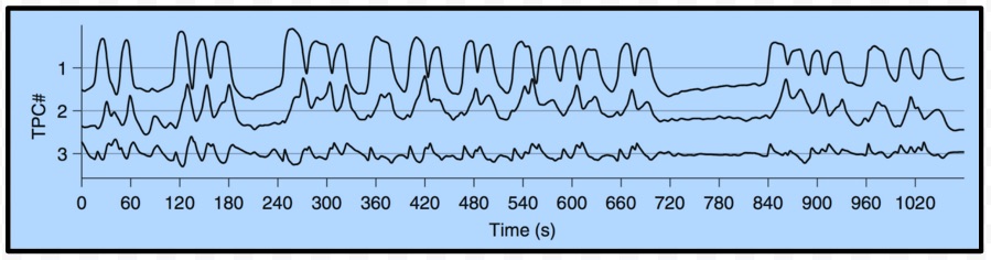
Temporal PCs as weighted sum of refactored time series⁴⁷;
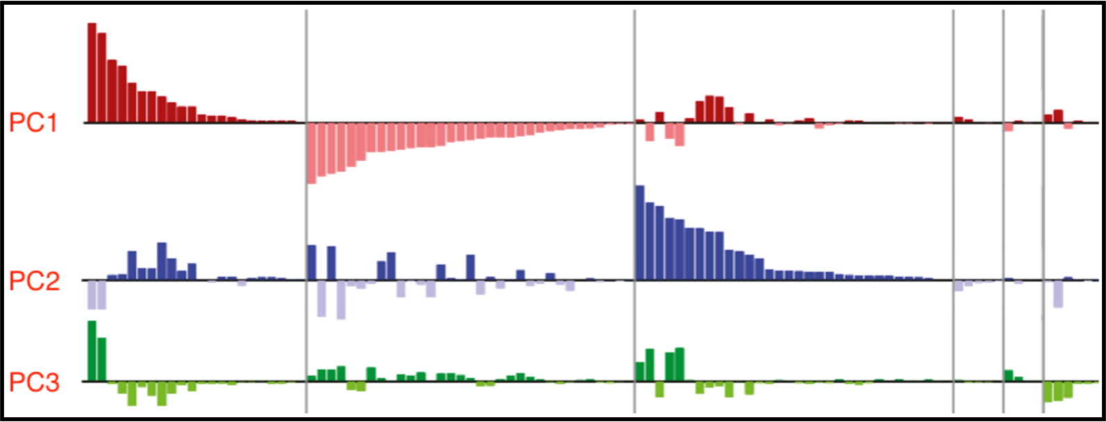
Cluster temporal PCs grouping highly correlated neurons:

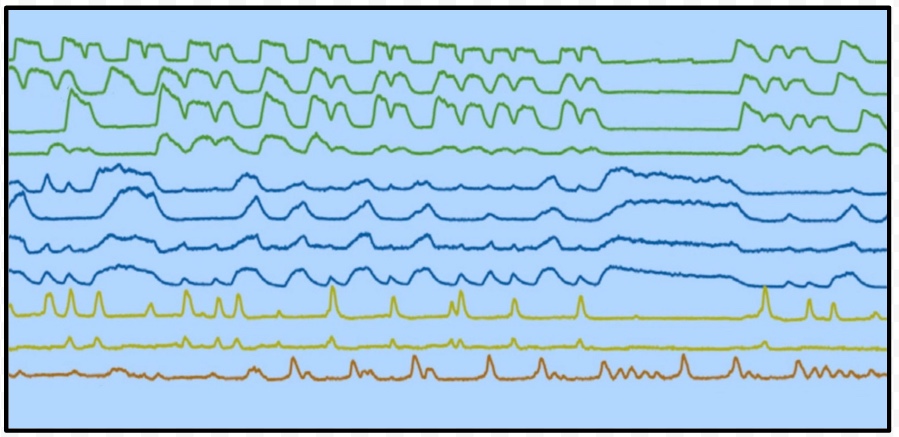
System evolves on low-dimensional, attractor-like manifold:

Ca²⁺ 2PE unconstrained imaging with IR behavior tracking;
Identify transitions and segment the time-series vectors:
Bundle repeated segments and construct the phase portrait;

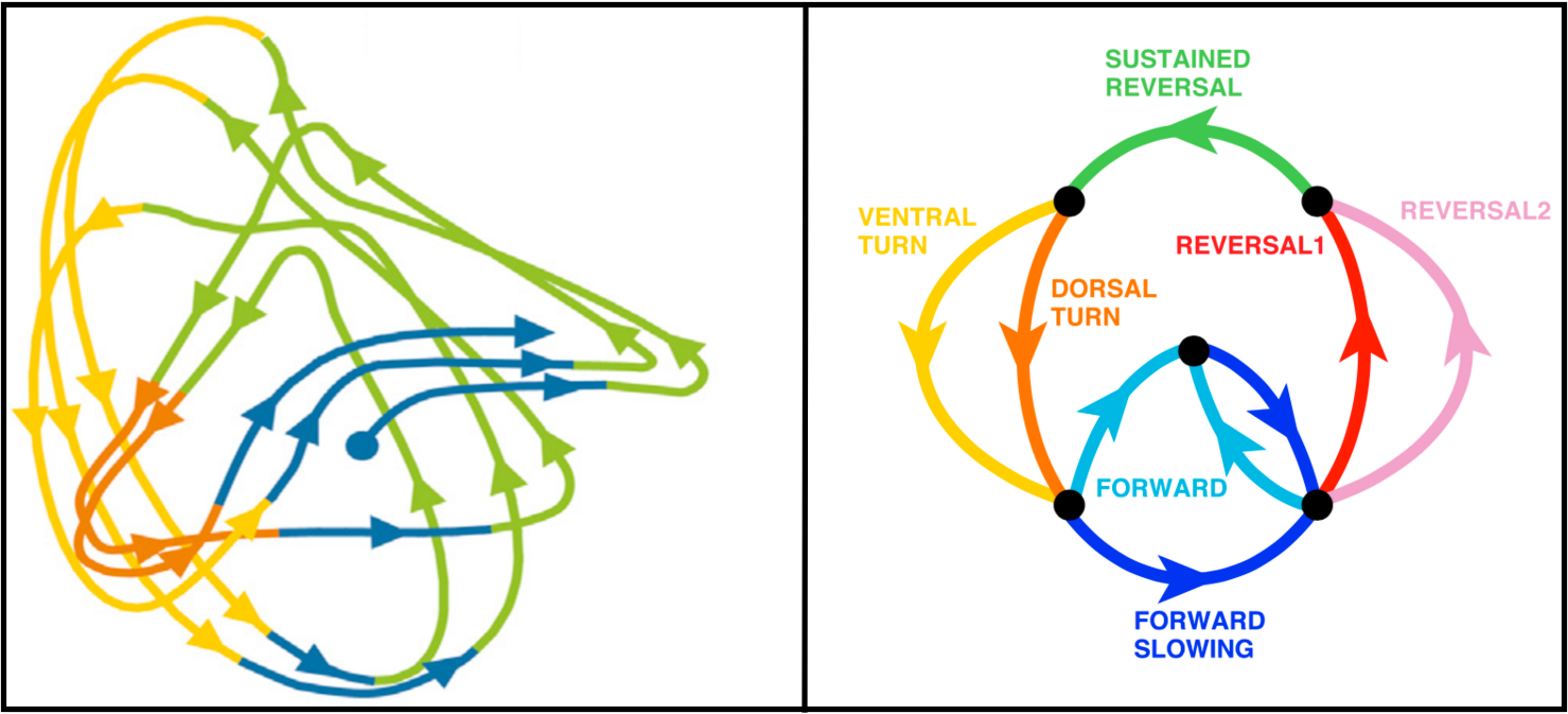
February 25, 2016

This entry is a hodgepodge of commentary on coupled relaxation oscillators for explaining neural activity and building novel computing architectures, reviewing the evidence for the simplifying assumptions about neural computation that Raphael Yuste and I discussed earlier this month—see here, and the content for two slides destined for the Cambridge University lecture at the Computational and Biological Learning Lab in March.

Making the Case for Simplicity

Here is Carver Mead [171] describing the fabrication of an artificial retina that takes advantage of some of the shortcomings of CMOS transistors—shortcomings in that they render such devices difficult to use in digital circuits⁴⁸. The italicized text characterizes neural circuits as being built out of components that have a lot of associated garbage and yet perform useful information processing:

We have designed a simple retina and have implemented it on silicon in a standard, off-the-shelf CMOS (complementary metal-oxide semiconductor) process. The basic component is a photoreceptor, for which we use a bipolar transistor. In a CMOS process this is a parasitic device⁴⁹, that is, it's responsible for some problems in conventional digital circuits. But in our retina we take advantage of the gain of this excellent phototransistor.
There's nothing special about this fabrication process, and it's not exactly desirable from an analog point of view. Neurons in the brain don't have anything special about them either; they have limited dynamic range, they're noisy, and they have all kinds of garbage. But if we're going to build neural systems, we'd better not start off with a better process with, say, a dynamic range of 10⁵, because we'd simply be kidding ourselves that we had the right organizing principles.

If we build a system that is organized on neural principles, we can stand a lot of garbage in the individual components and still get good information out. The nervous system does that, and if we're going to learn how it works, we'd better subject ourselves to the same discipline.

As in a biological eye, the first step is to take the logarithm of the signal arriving at the photoreceptor. To do this, we use the standard trick of electrical engineers, that is, to use an exponential element in a feedback loop. The voltage that comes out is the logarithm of the current that goes in. We think this operation is similar to the way living systems do it, although that is not proven. The element that we use to make this exponential consists of two MOS transistors stacked up. A nice property of this element is that the voltage range of the output is appropriate for subsequent processing by the kinds of amplifiers we can build in this technology.

When we use the element to build a photoreceptor, the voltage out of the photoreceptor is logarithmic over four or five orders of magnitude of incoming light intensity. The lowest photocurrent is about 10⁻¹⁴ amps which translates to a light level of 10⁵ photons per second. This level corresponds approximately to moonlight, which is about the lowest level of light you can see with your cones.

After more than a decade of studying neuroscience—more if you include the courses I took in graduate school, I'm only now really appreciating the scale and complexity of neural processes—especially at the molecular scale in which different physical laws dominate and the basic components are constantly undergoing change. No surprise that neurons have to work hard to harness the latent computing power in networks of neurons that individually and collectively exhibit such morphological diversity and physiological variability. I've been looking for other sources of corroborating evidence for our current working hypothesis.

Specifically, I've been reading papers on (i) the correlation among spiking neurons—especially complementary pairs of interneurons of opposite inhibitory / excitatory valence [12], (ii) the role of non-Gaussian noise and how adaptation and accommodation might be beneficial or not [49], (iii) whether correlated variance is redundant (maintaining information integrity) or additive (augmenting information content) [227, 235], and (iv) approaches focused on the synthesis of reliable organisms from unreliable components that go back to John von Neumann [260] as well as modern variants that focus on reliable computation from unreliable parts [30] (PDF). I've learned less than I had hoped for and hardly anything conclusive concerning our working hypothesis.

So apart from the considerable intellectual authority invested in Mead's comments, the most compelling source of evidence is the observations of theorists and modelers who have found that most of the variance found in the neuronal ensembles they study can be accounted for by the first two or three principle components of the recorded time-series vectors (one for every recorded neuron) and the corresponding phase portraits appear to lie on similarly low-dimensional manifolds [134, 4].

Ergo (we wishfully conclude) that whatever is going on in and among the incredibly complicated neurons comprising these ensembles, the net task-relevant computational expenditure is relatively small when compared to the total expenditure of effort. Quod erat demonstrandum we can ignore much of the "garbage" if all we want to do is model said task-relevant computations—including, e.g., such generalized functions as "executive control", but we ignore it at our peril if we want to build reliable computers out of quirky, unreliable components like biological neurons. [Note: It is also well to keep in mind how our understanding of "junk" DNA has changed radically over the last decade.]

Evidence for Neural Simplicity

Here is the content for a one-slide, talking-points summary of the above argument:

... variance in firing rates across neurons is correlated^[1]

... correlated synaptic input drive current fluctuations^[2]

... modulating network coherence is important in attention^[3]

[1] S. Panzeri, S. R. Schultz, A. Treves, & E. T. Rolls. Correlations and encoding information in the nervous system. Royal Society B: Biological Sciences, 266(1423):10011012, 1999.

[2] E. Salinas & T. J. Sejnowski. Impact of correlated synaptic input on output firing rate and variability in simple neuronal models. The Journal of Neuroscience, 20(16):6193-6209, 2000.

[3] X. J. Wang. Neurophysiological and computational principles of cortical rhythms in cognition. Physiological Reviews, 90(3):1195-1268, 2010.

... lot of garbage in components and still it performs well^[4]

... first 2-3 principle components account for Ca²+ rasters^[5]

... system phase-portraits lie on low-dimensional manifolds^[6]

[4] Carver Mead. Neural hardware for vision. Engineering & Science, 1:2-7, 1987.

[5] S. Kato, ..., M. Zimmer. Global brain dynamics embed the motor command sequence of caenorhabditis elegans. Cell, 163:656-669, 2015.

[6] V. Mante, ..., W. T. Newsome. Context-dependent computation by recurrent dynamics in prefrontal cortex. Nature, 503:78-84, 2013.

Worms, Flies, Mice and Monkeys

Here is a one-slide capsule summary of existing or soon-to-be-available opportunities for applied mathematicians, computer-scientists, condensed-matter physicists and neuroscientists of all stripes to keep their hands clean and their lab coats smelling sweet and still be able to make major contributions to understanding the brains and nervous systems of animals across a wide range of uncharted complexity. Here we consider only worms, flies, mice and monkeys:

Data Types:	EM structural; 2PE functional; IR behavioral; AT genomic^[1]
Annotations:	3D microcircuit reconstruction; sparse, weighted adjacency matrix
	boundary I/O: sensory / motor; afferent / efferent; axonal / dendritic
	neuron morphological types; synaptic coordinates & connection types
	dense GECI and GEVI fluorescence time series; neuron-indexed rasters^[2]
	directed clique-complex structure summarizing local circuit motifs
	barcode summary representation of persistent-homography evolution
Organisms:	species name — common name — target task — target volume
Experiments:	C. elegans — nematode — forward / backward motions — whole organism
	D. melanogaster — fruit fly — threat detection — medulla of optic lobe
	M. musculus — house mouse — vibrissal touch — somatosensory (barrel) cortex
	M. mutatta — rhesus macaque — various — whole retina, prefrontal cortex

[1] Biological microscopy technology: electron microscopy (EM), two-photon-excitation (2PE), infrared (IR), array tomography (AT)

[2] Fluorescent physiological probes: genetically-encoded voltage indicator (GEVI), genetically-encoded calcium indicator (GECI)

Coupled Relaxation Operators

There has been resurgence in interest of late in using coupled relaxation oscillators⁵⁰ for modeling the behavior of ensembles of spiking neurons—see Wang [265] for good overview of the neurophysiological and computational principles of cortical rhythms, synchrony and oscillatory activity in large neural circuits—and designing highly-parallel neurally-inspired computing architectures [273, 57] and algorithms that could exploit this source of parallelism [50, 15].

Unlike some instantiations of neural computing, distributed oscillator systems, such as coupled semiconductor lasers and micro-electro-mechanical (MEMS) resonators, are cheap and easy to make [121]. Anticipating the need for scalable SPICE-like simulations to simplify and speed design, Fang et al [69] have developed a method of accelerating the simulation of oscillator based computing systems that "can predict the frequency locking behavior [of coupled oscillators] with several orders of magnitude speedup compared to direct evaluation, enabling the effective and efficient simulation of the large numbers of oscillators required for practical computing systems".

February 19, 2016

Borrowing the definition from [196], an abstract simplicial complex K is defined as a set K₀ of vertices and sets K_n of lists σ = (x₀,...,x_n) of elements of K₀ (called n-simplices), for n ≥ 1, with the property that, if σ = (x₀,...,x_n) belongs to K_n, then any sublist (x_i₀,...,x_{i_k}) of σ belongs to K_k. The sublists of σ are called faces.

We consider a finite directed weighted graph G = (V,E) with vertex set V and edge set E with no self-loops and no double edges, and denote with N the cardinality of V. Associated to G, we can construct its (directed) clique complex K(G), which is the simplicial complex given by K(G)₀ = V and

K(G)_n = { (v₀,...,v_n): (v_i,v_j) ∈ E for all i < j } for n ≥ 1.

In other words, an n-simplex contained in K(G)_n is a directed (n + 1)-clique or a completely connected directed sub-graph with n + 1 vertices. Notice that an n-simplex is thought of as an object of dimension n and consists of n + 1 vertices. By definition, a directed clique (or a simplex in our complex) is a fully-connected directed sub-network: this means that the nodes are ordered and there is one source and one sink in the sub-network, and the presence of the directed clique in the network means that the former is connected to the latter in all the possible ways within the sub-network.

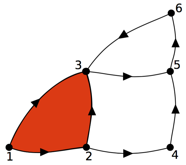Figure 23: The directed-clique complex corresponding to a directed-graph representation of a neural circuit. The directed-clique complex of the represented graph consists of a 0-simplex for each vertex and a 1-simplex for each edge. There is only one 2-simplex (123). Note that 2453 does not form a 3-simplex because it is not fully connected. 356 does not form a simplex either, because the edges are not oriented correctly—meaning in this case that the 356 subgraph does not have (exactly) one sink and one source [From Masulli and Villa [196]]

Masulli and Villa [196] and Dlotko et al [60] use essentially the same method of constructing the directed clique complex—Dlotko et al call it a directed flag complex—which isn't surprising given that Masulli and Villa got the idea of using ordered cliques to define simplices in a directed graph from Kathryn Hess, Ran Levi and Pawel Dlotko. There a number of other similarities between the two papers, e.g., the use of Betti numbers and Euler characteristics as the topological invariants in their respective analyses. They use interestingly different classes of random graphs as controls to verify that their models exhibit the expected connectivity patterns,

Both compare with Erdös and Rényi [67] random graphs. Masulli and Villa also compare with scale-free⁵¹ and small-world graphs [183]. Dlotko et al use a somewhat more nuanced, data-driven approach by randomizing the structural matrix of one of the average microcircuits from their reconstructions, taking into account its biologically meaningful division into six layers in 10 cases and into 55 morphological neuron types in 10 cases.

The tutorial on connectomic analysis focusing on topological and spatial features of brain networks by Marcus Kaiser [128] relies on purely graph-theoretic features and conceptually simpler methods of analysis, but employs a richer representation of directed graphs allowing a wider range of circuit motifs. In particular, it allows for bi-directional dependencies between vertices—there can be one, two or zero edges between a pair of vertices—and a less restrictive characterization of functionally-relevant sub networks—there is no requirement that a circuit motif (analogous to an n-simplex in the case of the other two papers) have a single source and a single sink. Figure 24 illustrates the advantages of this more expressive representation.

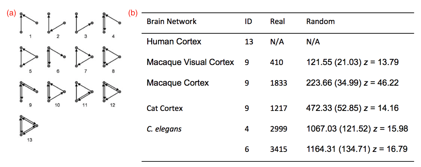Figure 24: Network motifs⁵² defined as frequently appearing patterns of connectivity predictive of functional roles. (a) Overview of all 13 possible ways to connect three nodes (three nodes without connections are not considered). (b) Three-node patterns that occur significantly more often in the human [120], macaque, cat, and C. elegans structural connectivity than in rewired⁵³ networks are network motifs. The ID numbers refer to the numbers in (a)). [From Kaiser [128]]

Note that only the C. elegans analysis was performed on a network of neurons since C. elegans is the only organism for which we have the complete connectome. During Andrew Leifer's visit, Bret Peterson was reminded of John Miller's work on crickets in which each neuron behaves like a collection of independent segments that operate autonomously [54]. Brett asked Andrew if he thought this was happening in the nematode, and Andy replied that it wasn't clear if we were dealing with 302 neurons or a thousand compartments.

The rest of the analyses were done using anatomical connection probabilities (ACP) between cortical and subcortical brain regions estimated with diffusion-weighted Magnetic Resonance Imaging (DW-MRI) techniques to trace major pathways consisting of bundled myelinated axons. The resulting graphs are undirected. If you're interested in this line of research, you should read the original papers by Milo et al [175], Sporns, Kötter and Tononi [237, 238, 236], and Iturria-Medina et al [120].

Given the differences in the nodes—neurons versus regions—and edges—synapses and the axons and dendrites they connect versus tracts corresponding bundles of myelinated axons—of their respective graph representations, it may be that they exhibit very different motifs. On the other hand, there is some evidence that the brains or parts of the brains of mammals exhibit some degree of self-similarity⁵⁴ in which case we may find examples of the motif labeled 13 in Figure 24.a at multiple scales in mammalian connectomes [206].

February 17, 2016

David Duvenaud introduced me to Guillaume Hennequin, Máté Lengyel and Daniel Wolpert in the Computational and Biological Learning Lab at Cambridge, and they invited me to give a talk and spend the afternoon on my stopover in London returning from Zurich. Guillaume, who is my host, asked for a description of my talk and I supplied the title and abstract below sans footnotes and citations.

When I sent it, I pointed out that I had attempted a little neuroscience humor in the title and a little hyperbole in the abstract, and that if staid and understated was the norm for talks at CBL, to please advise me and I would produce something more appropriate. Guillaume replied that it "looks great and will appeal to many here at CBL", so I guess I'm stuck with it. I kind of like it, but now I have to deliver on its promises or the jokes will fall flat and the hyperbole will be just that.

It's the Network Dummy: Exhuming the reticular theory⁵⁵ while shoveling a little dirt on the neuron doctrine⁵⁶

Scott McNealy, former CEO of Sun Microsystems, is rumored to have quipped⁵⁷, "It's the network dummy", when a reporter asked where the computer was upon seeing a room full of thin-client, diskless workstations⁵⁸. McNealy's point was that the power of computer networks isn't the (linear) sum of individual computers; the power is in the (nonlinear) manner in which they work together⁵⁹. When a computational neuroscientist examines an EM image of neural tissue, does she see a network or a bunch of neurons? The answer will depend on what she understands to be the fundamental unit of neural computation?

We assume the fundamental unit of neural computation is not the individual neuron⁶⁰, compartment, synapse or even circuit in the traditional sense in which electrical engineers generally think of circuits, but rather dynamic ensembles of hundreds or thousands of neurons that organize themselves depending on the task, participate in multiple tasks, switch between tasks depending on context and are easily reprogrammed to perform new tasks. Consequently, the total number of computational units is far fewer than the number of neurons.

We also assume that much of what goes on in individual neurons and their pairwise interactions is in service to maintaining an equilibrium state conducive to performing their primary role in maintaining the body and controlling behavior⁶¹. This implies that the contribution of small neural circuits to computations facilitating meso- or macro-scale⁶² behavior is considerably less than one might expect given the considerable complexity of the individual components. Since much of the complexity will manifest itself in the topology of the network, we need some means of computing topological invariants at multiple scales in order to tease out the computational roles of the multitude of circuit motifs⁶³ that are likely present, even in those parts of the brain assumed to be structurally and functionally homogeneous.

In the talk, we describe the convergence of several key technologies that will facilitate our understanding of neural circuits satisfying these assumptions. These technologies include (i) high-throughput electron microscopy and circuit reconstruction for structural connectomics, (ii) dense two-photon-excitation fluorescent voltage and calcium probes for functional connectomics⁶⁴, and (iii) analytical methods from algebraic topology⁶⁵, nonlinear dynamical systems⁶⁶ and deep recurrent neural networks for inferring function from structure and activity recordings.

February 15, 2016

Finished the 3rd and final installment on algebraic topology and persistent homology for functional and structural analysis of cortical neural circuits using as my running example the Dlotko et al [60] analysis of the reconstructions in Markram et al [166, 205, 209] — Henry is the first or last co-author on all of these papers. This follows on the heels of a similar appraisal of techniques from nonlinear dynamical systems theory using as a running example the Kato et al [133, 134] analysis of data collected in Alipasha Vaziri's lab and described in Schrödel et al [220]. Special Thanks to Costas Anastassiou, Surya Ganguli, Andrew Leifer, David Sussillo and Emanuel Todorov for feedback and paper suggestions.

Miscellaneous loose ends: Raphael Yuste dropped by last Wednesday and we had an interesting discussion. It seems Raphael and I share a frustration with cell biologists obsessed with the neuron, and attitudes among neuroscientists that either (a) we already know enough about neurons to construct elaborate theories about their individual contributions in specific circuits, or (b) it will be a long time — and a great many federal dollars — before we know enough to justify attempts to understand circuits of any complexity.

I agree with those in the (a) camp that there is value in trying to understand how small circuits work as long as we keep in mind the provisional status of current theories. (There is no reason to believe that just because we've been trying to understand neurons for over a century, the things we've come up with are the most important things to know.) I also agree with camp (b) that there is much to learn about individual neurons and some of what we learn will no doubt overturn existing theories about circuit function.

Raphael and I also share the intuition that the fundamental unit of neural computation is not the individual neuron, compartment, synapse or even circuit in the traditional sense in which most electrical engineers and many neuroscientists think of circuits, but rather ensembles of hundreds or thousands of neurons that organize themselves depending on the task, can participate in multiple tasks and switch between them depending on context and can be easily adapted / reprogrammed to perform new tasks.

This isn't true of all organisms and even in primates there are networks in which neurons behave more like the discrete components in an electrical circuit, but it probably is true of the neocortex. Raphael and I talked about the possibility that much of what goes on in individual neurons and their pairwise interactions is in service to maintaining some sort of equilibrium state conducive to performing their primary computational roles in maintaining the physical plant and controlling behavior.

Such a division of labor, say 90% to routine maintenance and homeostatic regulation at the microscale and 10% to computation required to conduct business at the macroscale, makes sense when you think of the lengths that semiconductor process engineers have to go to in maintaining the purity of the crystal substrate, precise depth of resists, diffusion of dopants, constant width of traces and vias, etc. Intel takes care of all this in production, the brain builds fragile, pliant neurons and never stops tinkering with them.

At least that's my current working hypothesis. It has both a scientific and pragmatic rationale. Pragmatic because if every neuron plays a unique role, we probably will need another decade to understand the neuron at the molecular level well enough to have any chance of unraveling the basis of neural computation. Scientific ... well, that would take too long elaborate on here, and I'm the first to admit that wishful thinking does play some role. I don't know if that makes me an optimist, pessimist or opportunist, but we all have to place our bets if we're to make any progress.

February 11, 2016

This installment focuses on analytical techniques from algebraic topology⁶⁷ that have started appearing in computational neuroscience papers on neural coding and dynamical systems. The discussion revolves around the representation of neural circuits as simplicial complexes, characterizations of such complexes using topological invariants, analytical tools including persistent homology and the application of these ideas to learning the connectivity and function of biological networks. I've tried to be conceptually clear and mathematically precise, using footnotes to supply formal definitions and references as needed⁶⁸.

The first step in applying these techniques is to represent a neural network as a directed graph G = (V, E) in which the vertices V (nodes) correspond to neurons and the edges E (connections) correspond to synapses, possibly weighted by strength or activity if there is data to support such an assignation. This graph representation is useful for static, structural analyses. If we have neural activity data, e.g., calcium imaging time series, we can apply this data to create a sequence of edge weighted graphs { G_t : 0 ≤ i ≤ T } representing the evolution of G over time in order to perform functional analyses.

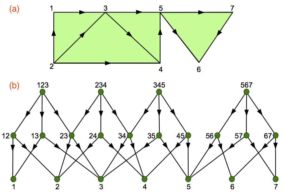Figure 21: Example of a simplicial complex and its corresponding Hasse diagram. (a) The geometric realization of a simplicial complex consisting of seven 0-simplices (labeled 1,...,7), ten 1-simplices, and four 2-simplices. The orientation on the edges is denoted by arrows, i.e., the tail of an arrow is its source vertex, while the head of an arrow is its target. (b) The Hasse diagram corresponding to the simplicial complex above. Level k vertices correspond to k-simplices of the complex and are labeled by the ordered sets of vertices that constitute the corresponding simplex. Note that, e.g., vertex 23 is a back face of a vertex 123 and a front face of a vertex 234. [From Dlotko et al [60]]

The next step is to summarize the subgraphs—neural circuits—of G as a simplicial complex. For our purposes, a simplicial complex representing G is the set of all subgraphs of G that are, in a restricted sense, complete, i.e., fully connected. The restricted sense is that, in order to create a canonical representation, we impose an ordering > on V and define a complete graph K consisting of n nodes in the underlying undirected graph to be an (ordered) directed n-simplex of G, if for each directed edge n_i → n_j in K, then n_j > n_i. The simplicial complex (SC) associated with G consists of all n-simplices for all orders, i.e., all n such that 0 ≤ n ≤ | E | — see the example simplicial complex shown in Figure 21.a⁶⁹.

Many of the recent papers in mathematical neuroscience⁷⁰ employ topological invariants to gain insight into simplicial complexes. Generally speaking, a topological invariant is a number that describes a topological space's shape or structure regardless of the way it is bent or twisted⁷¹. Euler chracteristics and Betti numbers are two such invariants. The Euler characteristic of a graph is the number of vertices minus the number of edges. The Euler characteristic of a simplicial complex equals the alternating sum, χ = k₀ − k₁ + k₂ − k₃ + …, where k_n denotes the number of n-simplexes in the complex. The Betti numbers are used to distinguish topological spaces based on the connectivity of n-dimensional simplicial complexes. The n^th Betti number represents the rank of the n^th homology group, denoted H_n, which tells us the maximum number of cuts that must be made before separating a surface into two pieces or 0-cycles, 1-cycles, etc.

That was all pretty abstract and so you're probably wondering when we're going to get back to talking about brains. Unfortunately, we still have some concepts and definitions to go. If you feel you could use a quick, Khan-Academy-style review and peek ahead, you're in luck — check this out. [...] For you intrepid remaining travelers or those rejoining us after watching Matthew Wright's quirky video, the next step is to describe how to construct a simplicial complex and its associated Hasse diagram. A Hasse diagram is a directed acyclic graph representing a partially ordered set (poset). Figure 21.b shows the Hasse diagram associated with the simplicial complex in Figure 21.a.

To follow the constructions described in the supplement of [60] would take us into some pretty esoteric realms of algebraic topology. Under the abstract simplicial complex genus, you'll find an array of subtly different species including clique complexes, flag complexes and conformal hypergraphs all of which describe the complete subgraphs of an undirected graph. Of course the algebraic topologists wouldn't consider the differences between species subtle, and so require several pages of definitions and lemmas to derive an abstract simplicial complex that can account for the variability found in the subgraphs of a directed graph.

In the case of [60], the result is a flag complex. A finite simplicial complex Δ is called a flag complex if every set of vertices that are pairwise joined by edges in Δ is a face of Δ. The finite sets that belong to Δ are called faces of the complex, and a face Y is said to belong to another face X if Y ⊂ X. For instance, every simplicial complex of all chains in a finite poset (partially ordered set) is a flag complex. In working with directed graphs, a face corresponds to an ordered set and has a geometric interpretation as a polyhedron.

The culminating result of the construction detailed in the Supplementary Text of [60] is the directed flag complex associated with the directed graph G defined as the abstract simplicial complex S = S(G), with S₀ = V and whose n-simplices S_n for n ≥ 1 are (n + 1)-tuples (v₀, ..., v_n), of vertices such that for each 0 ≤ i < j ≤ n, if there is an edge in G from v_i to v_j.

The authors then present the algorithm listed in ST2.3 of the Supplementary Text which takes as input the graph G of the neural circuit supplied in the form of an admissible Hasse diagram and produces as output the directed flag complex associated with G in the form of second Hasse diagram. The associated data structures facilitate efficiently adding and deleting edges in the graph thus altering the neural circuitry, updating the Hasse diagram to reflect those changes and computing Euler characteristics and Betti numbers that summarize the interleaved neural circuits and their respective interdependencies.

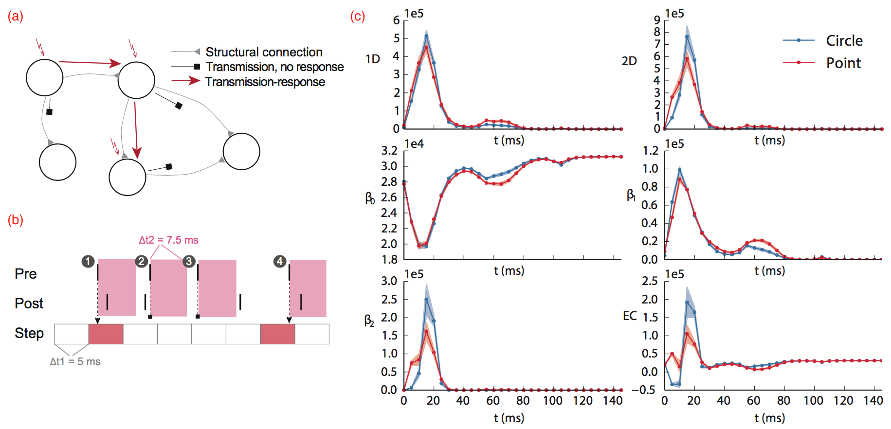Figure 22: The transmission-response paradigm for studying functional topology. (a) Schematic representation of the transmission-response paradigm: there will be an edge from j to k in the graph associated to particular time bin if and only if there is a physical connection from neuron j to neuron k, neuron j fires in the time bin, and neuron k fires at most 7.5 ms after the firing of neuron j. Here, shading indicates the error of the mean. (b) Schematic representation of those firing patterns involving a presynaptic and a postsynaptic neuron that lead to an edge in the transmission- response graph, with a red block indicating successful transmission and a white block indicating lack of transmission. (c) Time series plots of the average value of the metrics 1D (number of 1-simplices), 2D (number of 2-simplices), 0 (the zeroth Betti number, i.e., the number of connected components), 1 (the first Betti number), 2 (the second Betti number), and EC (the Euler characteristic) for the Circle and Point stimuli⁷². Here, shading indicates the error of the mean. [From Dlotko et al [60]]

Sections 1 and 2 of [60] describe the authors analyses of the Markram et al [166] reconstructions investigating their structural and functional topology. I'm primarily interested in the latter in terms of evaluating the prospects of using algebraic topology to study functional connectomics. The functional topology results rely on simulating reconstructed microcircuit models as in [166] to produce transmission-response graphs. They describe the production process as follows:

Topological methods [...] enabled us to distinguish functional responses to different input patterns fed into the microcircuit through thalamo-cortical connections. We ran simulations of neural activity in one of the reconstructed microcircuits during one second, over the course of which a given stimulus was applied every 50 ms [...]. We then binned the output of the simulations by 5 ms timesteps and associated to each timestep a transmission-response graph, the vertices of which are all of the neurons in the microcircuit and the edges of which encode connections in the microcircuit whose activity in that time step leads to firing of the postsynaptic neuron.

The result is a sequence of 200 transmission-response graphs G = { G_t : 0 ≤ i ≤ T } with T = 200. I can't improve on the discussion in Section 2 Functional Topology of the main text, so I suggest you read that portion of the paper and, if you haven't already, check out the Matthew Wright tutorial on persistent homology, not because it is directly relevant to Dlotko et al [60], but rather for a graphic and imagination-stimulating example of what one might do with sequences of simplicial complexes like G using analytical techniques akin to persistent homology.

Why not follow Raphael Yuste's lead and stick to simpler, off-the-shelf tools like principal components analysis, local linear embedding [218, 217] and stochastic variants like [110]? One reason is that these tried-and-true tools won't automatically exploit the intricate patterns of connectivity at multiple spatial scales that we believe to be a key feature of neural computation. Of course, these tools — or others in the machine learning repertoire — might be able to learn how to exploit such patterns. However, we might also end up reinventing flag complexes, stratified Hasse diagrams, Euler characteristics, Betti numbers, and other techniques in the algebraic topologist's toolkit.

I expect the tools in the ML repertoire and those in the algebraic topology toolset will complement one another and we'll learn to apply them when appropriate along with other tools we have borrowed from differential calculus, control theory, nonlinear dynamical systems, statistical mechanics, etc. Given recent success in mapping very-high-dimensional data to low-dimensional manifolds, one might ask why we don't we just train deep recurrent neural networks on inputs and outputs directly from the calcium imaging rasters as suggested earlier here and here. I still think this would be a powerful methodology given the neural network technologies we can bring to bear from research at Google.

There is growing literature on applying techniques from algebraic topology to neuroscience. I've included a small sample⁷³ of the papers — BibTeX entries including abstracts — I came across while working on this log entry. If you read nothing else referenced in this note, I suggest you read Markram et al [166] if you haven't already and then make a best effort to work your way through the Dlotko et al [60] assisted by the material in this and the previous log entries. Whether or not you ever use the techniques described in this paper, I expect you'll gain insight into the problem of inferring function from recordings of neural activity and the role structural connectomics might play in solving the problem.

Further Reading: The relevant sub field of algebraic topology is called Computational Topology. Gunnar Carlsson and Herbert Edelsbrunner are two mathematicians who have made major contributions to this field. The graduate-level text by Edelsbrunner and Harer [64] (PDF) provides a comprehensive introduction. Edelsbrunner and Harer's survey of the field [63] is a little dated but still useful as an introduction for someone just starting out. Gunnar Carlsson's introduction to topological data analysis[43] is highly relevant (PDF) and he is co-author of one of the earliest papers I read applying persistent homology to the analysis of the activity of neural populations in visual cortex [232].

Giusti has compiled a bibliography of papers that apply algebraic topology to neuroscience (BIB). Curto's topological analyses of neural codes [55] and her papers on hippocampal place and grid cells (BIB) provide additional examples of algebraic topology applied to neuroscience. In one analysis [90], Giusti, Curto and their colleagues use sequences of Betti numbers to provide a summary of the topological features of the matrix C_ij indicating the strength of correlation or connectivity between pairs of neurons in a particular circuit.

You'll encounter a lot of definitions and unfamiliar mathematical objects if this is your initial exposure to algebraic topology. I thought I knew a good deal about the subject given my background, but I struggled early on reading the journal papers. If you're diving into the field for the first time, I highly recommend you watch the YouTube video entitled "Introduction to Persistent Homology" by Matthew Wright (MP4). The animations are worth the time even if you're an expert in the field. It would have saved me a lot of time and frustration had I watched this before I started out last week. It isn't a substitute for the math by any means, but, in less than eight minutes, you'll learn what simplicial complexes and filtrations are and why persistent homology is useful for data analysis.

February 9, 2016

In an earlier entry in this log, I suggested we think of DRNNs as precision tools — akin to a set of lock picks, that one can use to probe, pick apart and unlock the functional composition of complicated nonlinear dynamical systems. Each DRNN is a pattern corresponding to a class of functions that can be fit to a dataset with varying degrees of success, providing functional and structural explanatory value in proportion to its specificity and ability to reproduce the observed input-output behavior. It might be argued that we're trading one black box for another, equally opaque representation. However, while we now routinely build deep networks with thirty or more layers most of which we have no idea how they contribute to overall performance, the layers themselves are relatively easy to understand individually, e.g., convolution, sigmoidal activation, half-wave rectification, various pooling and normalization operators are all pretty well understood.

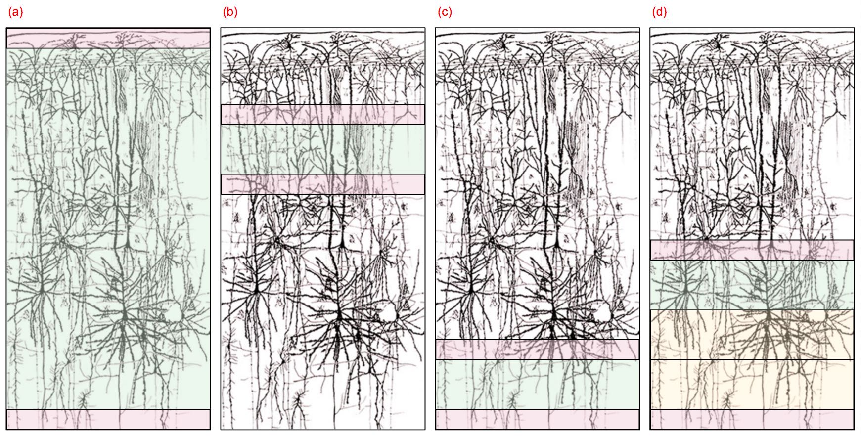Figure 19: Different approaches to training multi-layer cortical models from calcium imaging data. Color Key: green = the part of the neural circuit that you are trying to model, pink = the inputs and outputs of the target circuit specifying the Ca²+ traces to be used for training and testing, orange = previously trained portions of a multi-layer neural network being trained one layer at a time. We might (a) train a model of the entire circuit, (b) isolate and train sub-circuit models to use as components in a larger network, (c) train a deep network one layer at a time starting with the first layer — start at the peripheral inputs and iteratively extend the model to account for a greater fraction of the entire circuit, and (d) having trained the first n layers, train layer n + 1 by feeding the CI data through the completed layers to obtain the input for training layer n + 1. Caveat: In case it's not already obvious, all of the "inputs" won't feed into the "bottom" of the tissue sample nor will all of the "outputs" feed out of the "top" of the sample. Figure 20 and the following paragraphs address this issue.

To employ DRNN-probes with greater precision it would be convenient if we could test whether a part of a larger circuit is performing the function of, say, a linear transformation or a nonlinear pooling of its input. To illustrate, I created the graphics shown in Figure 19, horizontally slicing a cortical stack into various pieces and fitting them separately in an attempt to account for their component functionality. The problem with this picture, as I alluded to in the caption and Adam Marblestone noted in his email, is that simple horizontal sectioning as illustrated in the cartoon isn't likely to correspond to any coherent functional division. However, what if we could define functional partitions in terms of deep structural and functional divisions evident in the connectomic and calcium imaging data? Pawel Dlotko, an algebraic topologist at the University of Pennsylvania, and his co-authors including Henry Markram have taken some initial steps towards making this feasible.

Simplicial complexes and multidimensional persistence are core concepts in algebraic topology and in topological data analysis of high-dimensional datasets including very large directed graphs⁷⁴. Peter Bubenik and Dlotko are developing the Persistence Landscape Toolbox to facilitate this sort of data analysis [32, 31]. In Dlotko et al [60], the authors have used this toolbox along with resources provided by the Neocortical Microcircuit Portal [205] to analyze the reconstruction and simulation of microcircuits consisting of neurons in the neocortex of a two-week-old rat as described in Markram et al [166, 209].

I need some more time to digest the mathematics⁷⁵ and its application to the problem that prompted my original inquiry; however, from a cursory read-through of the paper, Dlotko et al appear to provide a potential solution to the problem of dividing large circuits into tractable components. The analysis begins by constructing the directed graph corresponding to the reconstructed neurons and classified synapses. The subsequent workflow involves generating adjacency matrices for the reconstructed circuits, computing all directed cliques of a given size for different orders, constructing flag complexes which are instances of oriented simplicial complexes that encode all orders of the underlying directed graph in terms of n-cliques. Most of the algorithms are straightforward.

The beauty of this approach is that, once you've generated these mathematical objects, you can employ a suite of powerful analytical tools to reveal interesting structure and produce complementary mathematical abstractions based on functional analyses of the (simulated) recordings yielding insights into circuit function. The authors also include an interesting analysis in terms of random graphs — both the original formulation of Erdös and Rényi [67] and more recent formulations motivated by naturally-occurring random-graph structures in biological and social systems as well as man-made systems such as computer networks and hyperlinked documents [183, 5, 61, 29, 87, 226, 24].

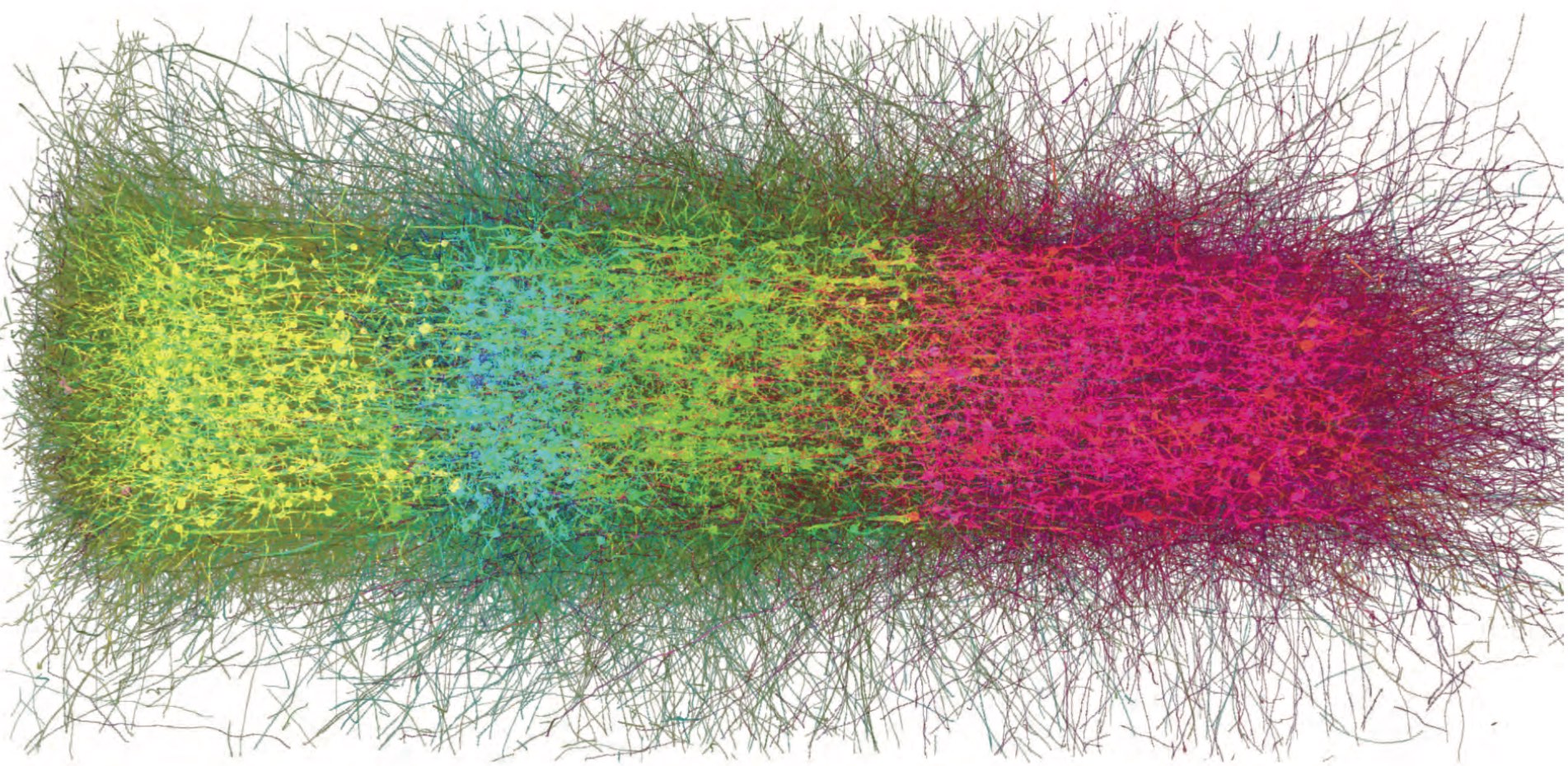Figure 20: An illustration of the divisions between layers in a DNN based on morphological cell type. (a) A sparse visualization of the microcircuit (showing soma and dendrites only). Morphological types are color-coded, with morphological types in the same layer having similar colors. [From Dlotko et al [60]]

The authors report that the topological analysis "revealed not only the existence of high-dimensional simplices representing the most extreme form of circuit motifs — all-to-all connectivity within a set of neurons — that have so far been been reported for brain tissue, but also that there are a surprisingly huge number of these structures." It is hard to visualize the implications of the results presented in this paper. Figure 20 is pretty much eye-candy, but it was the only image that conveyed some idea of what the division between functional layers might look like without requiring a lengthy and mathematically-detailed explanation of the graphic. It is worth pointing out however that the relevant level of abstraction is not at the level of individual neurons, but rather at the level of simplicial complexes. I plan to read the paper in more detail next chance I get and make a more concerted effort to convey why I think this is interesting and potentially relevant work.

February 7, 2016

I sent a note to Ed Boyden and Adam Marblestone asking for their feedback on the previous note. I've included below excerpts from their responses along with my replies. My exchange with Adam got me thinking about different approaches to training neural network models. I've included a quick note about this that I sent to Adam below and generated Figure 19 while watching the first half of the Super Bowl and the half-time show — first time for me hearing or seeing Beyonce, Coldplay or Bruno Mars ... I have to admit, however, that was a pretty cool giant display covering the entire stage. The caption doesn't have enough detail and I also want to come up with some different ways of exploiting the connectomic information in constructing model templates and training them.

Here are Adam's (AHM) and Ed's (ESB) responses to my request for feedback on the example functional-connectomics inference task:

AHM: Can you say a bit more about the example task? If I understand correctly, something like this is what you're proposing:

Take mm³ scale cortical calcium imaging datasets from MICRONS, and convert them to ~50,000 activity traces, one for each cell;

Train a RNN, say an LSTM, to predict the activity pattern at time T + n × Δ_t, given the activity pattern at time T − k × Δ_t, i.e., predict some window into the future given some window into the past

Use various regularizers on this RNN training process, to encourage the resulting RNN to be minimal in some sense;

You can then view the trained RNN as a description of the causal dynamics APPARENT in the calcium imaging data;

TLD: That's pretty much it. You use the accuracy of the predictions and various statistics on the inputs and outputs to judge how well you've captured the the dynamics. Some variant of the Cox et al high-throughput screening approach [199] for learning (searching for) high-performance models can be used for model selection.

Of course, there is no "hidden" state⁷⁶, if you believe that the Ca²+ levels are a reasonable proxy for the things you care about. Given that you can probe every synapse corresponding to a locus of fluorescent emission, you can carve out any sub circuit within the tissue sample, generate the corresponding CI rasters, and fit a model to just that sub circuit. The results of these experiments on "surgically isolated" circuit components could be used to construct a multi-layer model in a layer by layer by layer fashion — see Figure 19.
Of course, you could also replicate the entire connectome or any part in your RNN but then you're going to have to make a commitment to what's going on in the cell. Given the present state of our knowledge, we want to avoid modelling individual cells and bank on the idea that the wiring and proxy action potentials⁷⁷ in the form of fluorescent emissions can be modeled by some sort of standard ANN. That is to say, we don't really know how or what synapses and membranes compute but perhaps we don't need to if the connectome and CI rasters provide enough clues to summarize what's going on in suitably sized neuronal ensembles.

It would also be interesting to isolate ensembles of layer II/III neurons to try to mimic their behavior in a single LSTM layer. we know the behavior is recurrent, we expect it relies on keeping some state around, and we don't really have to know a priori which cells are excitatory and which are inhibitory ... though we might be able to infer this. If we record from an animal performing more than one task perhaps we can revisit the analyses in Surya's 2015 arXiv paper (Gao and Ganguli, 2015).

AHM: Using this you can (a) run the RNN predictor on activity data resulting different input stimuli or behavioral states to see how it generalizes, (b) analyze the low-dimensional structure of the RNN itself, effectively using the RNN outputs as a much larger set of "surrogate data" that is sampled from the same distribution, in some sense, as the original calcium imaging data, and of course comparing the low-dimensional structure of the RNN-generated surrogate data with that of the real data all the while, (c) play with different RNN architectures that are more or less similar to putative gross architectural features of cortex itself, (d) play with how various lesions to the data or to the architecture impact the ability to derive a causal model in this way.

TLD: Excellent. We're on the same page. Once you start thinking about, potentially there is a lot of science you can do, both exploratory and hypothesis driven.

AHM: You also seemed to suggest: using anatomical connectomes as an additional input to the RNN ... I didn't quite understand how that would fit in. ...

TLD: Haven't thought that through yet, but some of my comments above speak to the possibilities.

AHM: ... and training RNNs on C. elegans and Zebrafish datasets

TLD: One of the unintended consequences of partnering with several teams providing tissue samples and using different technologies is that we can serve as a clearing house for EM-related technology: keeping track of what stain, sectioning method, EM technology, etc is working best on what type of sample ... "here's how you might tweak your EM pipeline to make our learning algorithms faster, more accurate ... and as a consequence you'll get better reconstructions from us. Viren has a wide range of lab connections and he is a great at managing the various interactions.

As long as we can provide value, our highly motivated partners will continue give us valuable feedback ... we send them skeletons or full reconstructions, they check for errors, and give us the marked up sections back to serve as training data for the next round. By mixing data from different partners and different species, we get more robust models ... cross training improves generalization. If we build a better viewer or annotation tool or improve our infrastructure to serve, visualize or manipulate the data faster, then we get more / better ground truth, quicker turnaround. Lots of opportunity for virtuous cycles.

We can get data — CI rasters and EM data along with fiducials to help with alignment — for nematode, larval zebrafish, fly and mouse. Probably don't want all of these but we can be picky. After spending an afternoon with Andrew Leifer, I'm a convert to C. elegans; I think it would be exciting to work with him and interesting to apply the RNN-probe idea to analyzing worm circuits. And the Janelia fly data is super interesting — Peter is already working with Davi Bock, and we've been able to help him out on his project.

ESB: One of the biggest problems, as your notes suggest Tom, is how to monitor many physiological signals at once in a cell. We have a radical new proposal about how to do that: position indicators at different points in a cell, so that we spatially multiplex the measurements and can accordingly measure a great many things in a single cell. This will vastly help with then neuromodulator problem, which as you note applies to C. elegans, but probably applies to many other species too! The abstract for our spatial multiplexing project⁷⁸

AHM: In short, yes, I think this would be a tractable and fascinating approach to exploring the causal structure of large-scale activity mapping data at the present time, and very much worth the efforts of a few people in Google.

TLD: Thanks. We'll see what happens when I pitch the idea up my management chain.

AHM: It's also interesting to read your thoughts on the Kato and Ahrens activity maps and analyses. Yes, having behavior available, and knowing a lot about the neurons and circuits in those tiny organisms to begin with, is part of what makes this type of analysis possible. Using an RNN might allow you to attack cortical circuits without needing such detailed behavioral constraints, but then again, so might PCA. I would argue that even for the RNN approach, the tiny behaving organisms might be the right place to start, to test the basic principles.

ESB: Adam and I had a long chat recently with Saul Kato, of the Kato et al paper, about whether it might make sense to try to get the ground-truth datasets to "solve" the worm. And perhaps bring together modelers, scientists, technologists, and so forth. This could be very exciting.

TLD: Always good to experiment with PCA before invoking heavier machinery. PCA will handle / help approximate the linear sub units of behavior — the vector bundles, but the full model is most likely nonlinear — possibly approximated as piece-wise linear. Though I see your point; it's not uncommon to see papers that start with PCA to reduce the dimensionality to three or even two dimensions. If they're applying PCA correctly, then they are dealing with pretty simple behavior — Kato et al only dealt with a portion of the worms full repertoire ... they assumed movement was restricted to the plane even though worms lift their heads up for some activities — I think this was mentioned in one of Greg Stephen's papers.

AHM: Can you model C. elegans with fewer than 302 LSTM cells? If not, would that suggest that there are more than 302 bits of state in the system? Do you also need to add units that intrinsically oscillate, or that have more analog transfer functions, or different intrinsic timescales? If I run PCA on the activity states of the RNN trained on C. elegans, does that give the same manifold as what Kato found on the activity states of C. elegans itself? If not, why not?

TLD: All good questions / suggestions. As mentioned, we have a lot to learn from C. elegans and, contrary to what I used to think, it really matters very little that the neurons are not spiking. As for analog signals and organisms with spiking neurons, I can say there are LSTM models that can make sense of very small time intervals, but we don't have unlimited — or arbitrarily fast — computational resources and sampling a neuron in burst mode at twice the Nyquist frequency would be prohibitive even if we had a GECI/GEVI that could keep up pace. Then there are Maas' liquid state models — I keep meaning to check out some of his recent papers and get a Matlab or Numpy implementation to experiment with.

AHM: Best, Adam

TLD: Thanks loads for the careful read and great suggestions and questions.

February 3, 2016

This installment focuses on the functional connectomics⁷⁹. part of the AIBS collaboration [7]. Consider a cubic millimeter of mouse cerebral cortex or neocortex as it is commonly referred to in mammals—see Figure 12.b for an artistic rendering of a cube of brain tissue. There are on the order of 50,000 neurons in 1 mm³ of mouse neocortex⁸⁰ and about 1000 times as many synapses. The thickness of mouse neocortex varies in thickness—see Figure 17.d, but one millimeter is about average and so we'll assume our cubic millimeter sample extends through all six layers [250]. This is convenient given that the maximum depth of in vivo two-photon excitation microscopy in mouse cortex is ~1.6mm [142]. In theory, we should be able to record from all 50K of those neurons and so we'll assume this is true for the purposes of this discussion.

Figure 17: Brain mass, cortical thickness and gyrification. (a) The mouse brain is small (0.65 g) and is characterized by a smooth neocortex. The thickness of the mouse cortex is indicated by the colour scale. (b) By contrast, the human brain is considerably larger (1,230 g), and its cortex is gyrified. Its cortical thickness also varies but is, on average, thicker than that of mice. (c) The GI generally increases with brain mass across mammalian species for which data are available (n = 103). Manatees (Trichechus manatus (T.m.)) and humans (Homo sapiens (H.s.)) have relatively low GI scores for their brain mass compared with other mammalian species, such as the Atlantic bottlenose dolphin (Tursiops truncates (T.t.)). Other mammalian species not mentioned here are denoted by the blue data points. (d) Cortical thickness varies little with brain mass across species for which data are available (n = 42), except in manatees and humans, which have unusually thick cerebral cortices on average. [From Sun and Hevner [250]]

Clay Reid's team at AIBS will run a set of experiments with each mouse, recording Ca²+ levels—as illustrated in Figure 15.c—paired with time-stamped video of the visual stimuli being presented to the mouse, plus any additional information required for the subsequent analysis. Once the experiments are complete, the animal is euthanized, the cube of tissue is removed, sectioned and imaged, and the is connectome reconstructed and annotated.

To tie the structural and functional data together, the connectomic reconstructions and two-photon rasters are aligned, the fluorophore emission traces are mapped to putative synapses on the segmented neurons, pre-and post-synaptic neurons are identified within the connectome, and additional annotations are provided, possibly including proteomic assays, neuronal and synaptic classifications, excitatory-inhibitory designations, etc⁸¹. Once again, in theory, we can also assign inputs and outputs to the target block of tissue. Depending on the origin of the tissue, the accuracy of the alignments and the scientific focus of the experiments, the relevant input-output distinction may correspond to afferents versus efferents, dendrites versus axons, spines versus boutons, or sensory versus motor neurons.

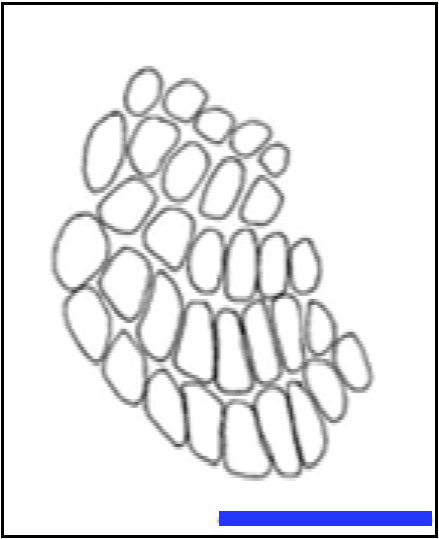Figure 18: Representative camera lucida⁸² drawing of the barrel field of a mouse. The mouse is a genotyped adult male wild-type (n = 3) provided to the authors [184] by Dr. C. Ronald Kahn at Harvard Medical School. The barrel field consists of a grid of cortical columns called barrel columns arranged in a spatial map serving a similar function to the retinotopically mapped regions of the visual cortex. Note that the blue scale bar is 1 mm indicating that a millimeter cube can easily encompass one or more barrel columns and all of their immediately adjacent neighboring columns. [From Guevara et al [184]]

Mice have limited color vision and relatively poor acuity which is probably associated with the fact they tend to live in subterranean environments. They rely heavily on their whiskers and keen sense of hearing to navigate in the dark [203]. In general, mouse cortex is much like the cortex of other mammals at least insofar as having the same basic six-layer architecture. Mouse facial whiskers, called vibrissae, supply the tactile extensions for their vibrissal sense of touch. Mice can move their whiskers so quickly that the vibrissae appear to vibrate, hence the Latin root vibrare meaning "to vibrate". Each facial whisker is associated with a dedicated cortical column, called a barrel column, located in the barrel field of the somatosensory cortex. The barrel field together with vibrissal touch and the ability of mice to sense their environment by precisely moving their vibrissae provide an ideal framework in which to study the function of cortical columns in the neocortex [71].

Ignoring for now the myriad technical details that I'm sweeping under the rug, imagine the following dataset modeled after the simulated data that Costas Anastassiou from AIBS shared with the students in CS379C last Spring. Basically there are two types of data files: one or more calcium imaging (CI) raster files and an annotated connectome (AC) dictionary file:

Each line in a CI raster file has the form: s, x_s, y_s, z_s, n_s,0, n_s,1, c_s,1, c_s,2, ... c_s,T, where s is the integer index for a synapse, ⟨ x_s, y_s, z_s ⟩ is the location of the synapse in the coordinate space of the reconstructed tissue sample, n_s,0 and n_s,1 are the indices of the pre- and post-synaptic neuron, respectively, c_s,t is the observed Ca²+ level in the pre-synaptic neuron at time t, and T is the number of samples in the time series.
Each line in the AC dictionary file has the form: n, u_n, v_n, s_n,1, s_n,2, ... s_{n,M_n}, where n is the integer index for a neuron and the label for voxels assigned to n in the reconstruction, u_n is the index for a neuronal type { 1, 2, ..., U }, v_n is the neuron's valence, −1 for inhibitory, 0 for unknown and + 1 for excitatory, s_n,1, s_n,2, ... s_{n,M_n} are the synapses such that n is the pre-synaptic neuron, and M_n is the number of such synapses for n.

What would you do with such a dataset? You could construct a recursive neural network using the specified inputs and outputs and train the model using backpropagation. This exercise would be worthwhile since (a) it hasn't been done before, (b) it is relatively straightforward to carry out, and (c) we'll surely learn something of value. For example, if you know something about the layered structure of the neocortex, you might recall that layer II/III consists of a network of excitatory and inhibitory interneurons and exhibits some intriguing dynamical behavior [83, 82]. Based on the structure of the sample connectome, you might experiment with a variety of deep recursive neural networks models to account for phase changes in the underlying dynamics of these interneurons or provide evidence for or against various hypotheses concerning the role of layer II/III interneurons in resolving ambiguity [140, 141, 174].

You can think of the DRNNs as a collection of precise tools, akin to a set of lock picks, that one can use to probe, pick apart and unlock the function of complicated nonlinear systems such as neural circuits. David Cox pioneered this approach with his high-throughput screening methodology [52, 17, 199] and Jim DiCarlo and Charles Cadieu are among a growing number of other neuroscientists applying similar approaches [161, 274].

While an artificial neural network isn't likely to satisfy most neuroscientists' interest in having an explanatory model of cortical function, if we think of the DRNN as nonlinear dynamical system reproducing the function of the original neural network, we can bring to bear a rich set of mathematical tools and computational techniques from the study of dynamical systems to construct a more satisfying account of the sought-after functionality [247, 251, 190]. We've already encountered one such exercise in David Sussillo and Omri Barak's method of recovering stable and unstable fixed points and inferring low-dimensional dynamics from high-dimensional RNN models [252].

I've provided just a few suggestions to get your creative juices flowing. If you have ideas for analyzing the sort of datasets described above—however wild and crazy those ideas might seem, please pass them along. Let a thousand flowers bloom. The more creative ideas we have, the more likely we are to stumble on one or two worth pursuing.

January 31, 2016

Technology for calcium imaging in awake behaving organisms has made extraordinary progress in just the last few years: from immobilized, whole organism imaging; to partially-constrained, whole-brain, single-cell resolution imaging [201, 200]; to freely moving, real-time tracking, whole-organism imaging with lab-on-a-chip chemical stimulus delivery [220]; to freely moving, real-time tracking, whole-brain, single-cell resolution imaging and precise single-cell optogenetic stimulation [185].

Recent innovations like the miniature (1.9 g) integrated fluorescence microscope that can be mounted on the skull of an awake behaving mouse [86] are enabling scientists to perform similar examples on mice. It is also possible to simultaneously record from two widely separated locations in the brain with two-photon fluorescence microscopy [148] or to conduct behavioral studies that combine experiments with a miniature microscope mounted on a freely-moving mouse recording on the order of 100 neurons with experiments on constrained animals using bench-mounted microscopes capable of recording from 1000 neurons or more [104].

The fluorescent indicators used in these experiments—called genetically encoded calcium indicators or GECIs—are also evolving quickly. GECIs can now detect single action potentials (APs). GCaMP6f [45] is the fastest variant in the latest iteration of calcium sensors with mean half decay times 142 ± 11 ms (1 AP, mouse V1 cortex), 400 ± 41 ms (10 APs, dissociated neuronal cultures) and ~650 ms (zebrafish tectum). But calcium is a proxy for what we're primarily interested in, namely, the direct readout of membrane potential changes. Furthermore, given that calcium transients can persist in neurons for hundreds of milliseconds, calcium responses cannot track high-frequency spike trains.

Genetically encoded voltage indicators (GEVIs) like ArcLight [124] offer the prospect of significantly faster tracking and direct measurement of local field potentials instead of relying on a (lagging) proxy in the form of calcium influx. ASAP1 (Accelerated Sensor of Action Potential #1) from Mark Schnitzer's lab has demonstrated on-and-off kinetics of ~2 ms, reliably detecting both single action potentials and subthreshold potential changes. ASAP1 has tracked trains of action potential waveforms up to 200 Hz in single trials [239].

As promised in the last entry posted in this log, what follows is a succinct explanation of the main steps described in [133] for deriving the Caenorhabditis elegans motor-control-system model: Refer to the previous entry for an introduction to dynamical systems modelling including the terminology used in the Kato et al paper appearing in Cell and two related papers that are introduced below. All three of these papers were recommended by Michael Hausser at the Wolfson Institute for Biomedical Research at University College London.

The data collected from 109 head neurons—see Figures 15.a-b—takes the form of a 109-dimensional time series of the recorded Ca²+ traces—see Figure 15.c. Perform principal components analysis (PCA) on the time derivatives of the normalized traces, and, for each principal component (PC), construct a temporal PC by taking a weighted average of the full 109-dimensional vectors that comprise the time series. The authors state that the temporal PCs represent "signals shared by neurons that cluster based on their correlations." If you read the supplement, you will be directed to a previous paper [134] for more detail concerning how these vectors were computed. Suffice to say that the first three PCs accounted for 65% of the variance in the complete time series and so {PC1, PC2, PC3} is taken as a basis for the model state space.

The phase plots of temporal PC1-3 shown in Figure 15.d indicate a cyclic process so that the repeated cycles form spatially coherent bundles. The neural state trajectories trace out a neural-state manifold corresponding to the subvolume in the transformed state space defined by the principal-component basis. The authors deconstruct PC1-3 to reveal how the most active neurons—typically combinations of motor neurons and opposing interneurons—at any given time work together or antagonistically to produce the behaviors observed at the corresponding times in experimental trials. This serves as a sanity check on the behavioural coherence of the model that would be difficult were it not for the wealth of information we have concerning C. elegans.

The authors then discuss how they derive a functional interpretation of the neural-state manifold by examining movies made with an IR camera while simultaneously performing calcium imaging—with a wavelength that doesn't interfere with IR camera—and targetting specific neurons based on their PC weights and the availability of promoters to drive expression of the fluorescent proteins. The remainder of the paper chronicles a rather complex analysis that combines rather subtle insights concerning the observed behavior and relevant biology with relatively simple methods for filtering, regularizing, segmenting and clustering the data to produce the phase diagram and state machine shown in Figures 14.d-e.

I don't mean to give the authors' behavioral and biological analyses short shrift — part of my reason for bringing it up at all is to underscore the fact that without such a careful analysis and decades of painstaking lab work there would be no objective measure to verify their model. The model is not—at least as presented in this paper—a predictive model and so cannot be judged on its accuracy in making extrapolations concerning consequences it was not explicitly trained to account for. It was not conceived of de novo but rather with the benefit and biases of generations of scientists chronicling every nuance of the worm's behaviour and the many biological pathways, genetic regulatory networks and neural circuits that make it possible.

There is a small but growing number of neuroscientists using similar combinations of dimensionality reduction and dynamical-systems modeling to explain behavior in various organisms. Niessing and Friedrich [187] develop a model of olfactory pattern recognition in zebrafish to test an hypothesis that computations involved in odour classification are carried out by switching between the activity (attractor) states of small ensembles of neurons in the olfactory bulb. Ahrens et al [4] present employ similar strategy to study how zebrafish generate motor activity and adapt it to changes in sensory feedback. Both papers offer explanatory models. An alternative approach might be to devise a predictive model that can be judged solely on its ability to predict unseen data⁸³.

Figure 15: Calcium-imaging data and state-space dimensionality-reduction method used in constructing Caenorhabditis elegans model. (a) Maximum intensity projection of a representative sample recorded under constant conditions. (b) Single z plane overlaid with segmented neuronal regions. (c) Heat plot of fluorescence (DF/F) time series of 109 segmented head neurons, one neuron per row. Labeled neurons indicate putative cell identifiers from the Worm Atlas. Ambiguous neuron IDs are in parentheses. Neurons are colored and grouped by their principal component (PC1-3) weights and signs, which are shown by the bar plots on the right. (d) Integrals of the first three temporal PCs. (e) Variance explained by first ten PCs, black line indicates cumulative variance explained. [From Kato et al [133]]

How is the cortex organized? Is there a single algorithm implemented with slight variation across the entire cortical sheet or is the cortex algorithmically more diverse? If we could simultaneously record from all the neurons in a cortical column [181, 198, 106, 113, 180, 179], could we infer the function being computed? Perhaps a cortical column is more like a multi-function pocket knife or a fully programmable gate array [163]? As much as we would like answers to these questions, attempts so far have not been convincing [137, 147, 85, 93, 105] and often the most capable mathematicians and computer scientists do not even attempt to find answers, opting instead to focus on well-defined data analysis problems such as spike sorting [191, 168, 258] and inferring connectivity from electrophysiology and calcium-imaging data [47, 178].

Deep feed-forward networks (DNNs) and their recurrent counterparts (RNNs) including LSTMs and more exotic models such as liquid-state machines, Hopfield networks and echo-state networks all have been claimed at one time or another to model computations in the brain. Whether or not these claims are true, DNNs and RNNs—corresponding to different classes of predictive models—have been demonstrated to perform well at learning complex input-output relationships and are being employed in neuroscience to test hypotheses concerning the foundations of biological computation [39, 38].

Mante et al [162] employ RNNs to explore an hypothesis that the prefrontal cortex (PFC) plays an important computational role in context-dependent behavior. The authors find that the (previously) puzzling responses of individual PFC neurons can be explained in terms of a dynamical process unfolding at the population level and succeed in training an RNN to reproduce the observed population dynamics. Yamins et al [274, 275] construct DNN models of the ventral visual stream to solve category-level object recognition problems that exhibit performance resembling both macaque inferotemporal (IT) cortex and human ventral visual stream⁸⁴.

I want to return to the problem of inferring the function being computed in a cortical column or other anatomically separable neural tissue sample. Having tried just about every sequence of relevant search terms I could think of and discovered little by way of a fresh approach that might actually work in the relatively near term, I went back a decade to see if much had changed in the intervening years. I read two survey articles [221, 101] in the special issue of Trends in Neurosciences on "Microcircuits" and scanned the abstracts presented at the 2006 Cold Spring Harbor workshop on "Neuronal circuits: from structure to function". There was a copy of a CSH technical report including all the submitted abstracts in the Stanford University library.

Figure 16. Neural circuits featured in [101]: (a) Hippocampal microcircuit — showing major cell types and synaptic connections in hippocampal CA3 region. (b) Neocortical microcircuit — showing major cell types and synaptic connections. (c) Cerebello-olivary microcircuit — showing the cerebellar cortex and its afferents. Common Key: Excitatory neurons are in red, inhibitory neurons are in blue, excitatory synapses are shown as V-shapes, inhibitory synapses are shown as circles and electrical synapses are shown as a black zigzag. Dashed circles depict afferent and efferent extracortical brain regions.

I found the examples in the De Schutter et al [221] paper—see Figure 16—representative of the dominant methodology of the time and of a style and at a level of detail still common today. One of the authors, Henry Markram, now works on large-scale simulations of biologically-realistic models. Markram's 2015 paper [166] describes a departure from the scale and methodology of a decade earlier—more in common with the Large Hadron Collider than what was and still is the norm in academic neuroscience. We could build better simulation tools capable of handling much larger models but the scientific contribution would be incremental at best. We'll explore some alternatives in the next installment.

Miscellaneous loose ends: As a handy reference in these notes, Table 1 lists the number of neurons in the brains of relatively large animals and in the entire nervous system in the case of the smaller animals. Table 2 lists the number of neurons in the cerebral cortex of some of those animals that have a cerebral cortex.

January 29, 2016

To get some idea of how many—if not most—neuroscientists thought about neural circuits in the 1980s and early 1990s, imagine pristine, well-separated, neurons suspended in the extracellular matrix and communicating with one another through unidirectional channels in a directed graph and data gleaned from sparse electrophysiology patch-clamp and multi-electrode-array (primarily) in vitro recordings. Fast forward to the present day and graduate students are learning to think of neurons as semipermeable bags exchanging molecules and fluids bidirectionally with one another through a bewildering array of different types of synapse and diffusely through the extracellular (interstitial) fluid and data collected (increasingly) in vivo with dense calcium imaging using GECI and GEVI and two-photon microscopy. The latter biological and technological perspectives reflect a better understanding of molecular and cellular structure and dynamics acquired over two decades of painstaking lab work and the stirrings of an exponential-growth process akin to Moore's law that has already achieved orders-of-magnitude increase in the number of neurons that we can simultaneously record from — see Figure 13.

Figure 13: Homage to Santiago Ramón y Cajal whose detailed studies, theoretical insights and scientific vision inspire neuroscientists to this day. The image on the lower right attempts — but fails miserably — to update the drawings of Cajal with highly schematic mechanical drawings that mask many of the important properties of neurons that we have discovered during the nearly 100 years since Cajal made his observations and meticulous hand drawings of cortical tissue samples.

Beginning with this entry and continuing for several more installments, the plan is to contrast—and better articulate—the following two (modernish) approaches to neural-circuit modeling:

model functional capability, e.g., face recognition, as a monolithic deep network — see the work on context-dependent behavior in PFC and LIP from Bill Newsome's and Krishna Shenoy's labs—Sussillo et al [252, 162]—and shape recognition in IT from Jim DiCarlo's lab [161, 39, 275]; it is relatively simple to build the models and run the experiments, the approach is inherently hypothesis driven, and the explanatory value is primarily at the the macro scale;
decompose a relatively large circuit into smaller component circuits using dimensionality reduction and nonlinear dynamical systems theory — see work on the persistence of orientation memory in C. elegans from Bill Bialek's group [242, 241] and the control-systems model for C. elegans coordinated motion from Manuel Zimmer's lab—Kato et al [133]; doing this well depends on careful analyses of the molecular and cellular mechanisms underlying behavior, the explanatory value at the meso scale [278];

Since it will prove useful in subsequent installments, we finish this entry with a short introduction to dynamical systems modelling. As mentioned in an earlier note, if you want more detail on dynamical-systems theory you might try Koch and Segev [144], Strogatz [247] and then Izhikevich [122] in that order. You might also want to check out the textbooks by György Buzsáki [36] (somewhat less challenging than [122]) and Bill Bialek [20] (somewhat more challenging than [122]).

Kato et al [133] use terminology from differential geometry and algebraic topology to describe their model. For the most part, anyone intuitively familiar with the concepts of manifolds, phase spaces⁸⁵, degrees of freedom⁸⁶ and vector spaces can understand the basic ideas. One possible terminological exception is the concept of a (vector) bundle⁸⁷ which is often encountered in mathematical papers on dynamical systems. You might also run into fiber bundles, stable bundles, principal bundles and other classes of bundles that you can often safely ignore if you simply want to understand the main conceptual contribution of a paper. For the most part, you can think of a bundle as a collection of state-space trajectories that characterize a behavior such as turning. The modeler has some leeway in deciding what constitutes a behavior, but in neuroscience the decisions generally revolve around the complexity of a proposed behavior and the coherence of the neural circuit hypothesized to produce it. A model builder might decompose one bundle—the "turning" bundle—into two separate bundles—one for "turning left" and another for "turning right"—if the associated behaviors employ different neurons to exercise different muscles.

Figure 14: The brain-wide activity of the C. elegans motion control system is organized in a low-dimensional, recurrent neural-state-space trajectory. (a) Phase segmentation of example AVAL⁸⁸ trace (left). Four-state brain cycle (middle). Phase timing analysis and clustering leads to six-state brain cycle (right). (b) Phase plot of the single trial shown colored by six-state brain cycle plus FORWARD_SLOWING command state in purple. (c) Phase-registered averages of the two RISE phase and two FALL phase bundles colored by six-state brain cycle. Semi-transparent ovals denote trajectory bundle mixing regions. (d) Contour surface illustrating the neural state manifold colored by six-state brain cycle. (e) Flow diagram indicating the motor command states corresponding to the six-state brain cycle plus FORWARD_SLOWING command state (purple). [From Kato et al [133]]

Bundles can be combined to represent complex behaviours by defining transformations that map one bundle into another. A collection of bundles along with a set of transformations that define the possible transitions between bundles can be used to represent the full behavioral repertoire of an organism. The result is a dynamical-systems model that can be concisely summarized as a (stochastic) finite state machine, as was done in the Kato et al [133] paper — see Figure 14.(e).

Miscellaneous loose ends: Michael Hausser at University College London suggested the Kato et al paper from Manuel Zimmer's lab at the Research Institute of Molecular Pathology in Vienna. Surya Ganguli suggested I go back to the papers out of Bill Newsome's and Krishna Shenoy's labs. I have some notes from my discussion with David Sussillo who is now at Google working in the Brain group. Check out the work of Greg Stephens, Bill Bialek and their colleagues and, in particular, the C. elegans analysis on page 7287 of [240] and the zebrafish analysis on page 5 of [80]. Finally, an apology to the reader is in order. This log entry is scattered and harder than some to follow. Unfortunately, there's no time to fix it now and it's unlikely I'll get back to it in the near future.

January 27, 2016

I asked Surya Ganguli if he had any good examples of non-linear dynamical-system models of whole organisms. Here's what he had to say:

TLD: Do you have a good example of a paper in which the authors fit a model to a dataset of the complexity of Andrew's data. Ideally a non-linear dynamical-system model that can be used to predict behavior and can be analyzed / explained in terms of lower-dimensional manifolds, attractor basins, etc.
SG: To my knowledge, there are not many good examples of what you ask for: nonlinear dynamical systems models of both neural activity (at whole brain level) and behavior that are both predictive and interpretable / explanatory. One interesting example is David Sussillo's work [162] with Newsome & Shenoy—where you fit behavior only and the internal dynamics of neurons look like what is found in the brain. However, this did not directly lead to new predictions/experiments as far as I last talked to them.

TLD: Thanks for the suggestion to check out David Sussillo's work. I imagine that research partially inspired your recent work with Peiran Gao that you presented in CS379C last spring [83].

SG: We know that the C. elegans behavior is low dimensional, four dimensions or so — see the work of Greg Stephens, Bill Bialek and their colleagues [242, 241]. So I think just very basic work characterizing the dimensionality and dynamics of neural activity, and then attempting to learn low dimensional dynamical models by connecting dimensionally reduced neural dynamics to dimensionally reduced behavioral dynamics might be a good first step, i.e. a coupled dynamical system of neural state space trajectories, and behavioral state space trajectories. With this in hand, one could look then look at relations between low dimensional representations of neurons/behavior, and understand how they map to the original high dimensional neural/behavioral parameter spaces. This breaks down the problem somewhat.

SG: One thing to be aware of is neuro-modulation, which is highly prominent in C. elegans but invisible to calcium imaging. Neuromodulators can sometimes even change the sign of synapses, as well as electrical circuit topology, so these unobserved degrees of freedom could present significant challenges to modelling calcium signals alone. I find Andy's work very exciting. Do keep me posted on efforts you guys make on this front. I am not working on this, so I would love to hear about it.

TLD: Thanks for the suggestions and pointers. Are you following the work of Manuel Zimmer? He's been collaborating with Vaziri. Michael Hausser sent me the attached Cell paper this morning [193]. I'm aware of the neuromodulation issue; it's one of the reasons that Ed Boyden is pushing his lab to extend Expansion Microscopy to label, locate, track, count, and collect statistics on every molecule possible.

Table 1: Number of neurons in the brain or whole organism in the case of the smaller animals (SOURCE):

Nematode roundworm	302	Caenorhabditis elegans — 7,500 synapses
Jellyfish	5,600	Hydra vulgaris
Box jellyfish	8,700-17,500	Tripedalia cystophora⁸⁹
Medicinal leech	10,000	Hirudo medicinalis
Pond snail	11,000	Lymnaea stagnalis
Sea slug	18,000	Aplysia californica
Fruit fly	250,000	Drosophila melanogaster
Larval zebrafish	100,000	Danio rerio
Lobster	100,000	Homarus americanus
Ant	250,000	Formicidae [various]
Honey bee	960,000	Apis mellifera — 10⁹ synapses
Cockroach	1,000,000	Periplaneta americana
Adult zebrafish	10,000,000	Danio rerio⁹⁰
Frog	16,000,000	Rana pipiens
Smoky shrew	36,000,000	Sorex fumeus
Short-tailed shrew	52,000,000	Blarina carolinensis
House mouse	71,000,000	Mus musculus — 10¹¹ synapses
Golden hamster	90,000,000	Mesocricetus auratus
Star-nosed mole	131,000,000	Condylura cristata
Brown rat	200,000,000	Rattus norvegicus — 5 × 10¹¹ synapses
Eastern mole	204,000,000	Scalopus aquaticus
Guinea pig	240,000,000	Cavia porcellus
Common tree shrew	261,000,000	Stavenn Tupaia
Octopus	500,000,000	Octopus vulgaris
Common marmoset	636,000,000	Callithrix jacchus
Cat	760,000,000	Felis catus — 10¹³ synapses
Black-rumped agouti	857,000,000	Dasyprocta punctata
Northern greater galago	936,000,000	Otolemur garnettii
Three-striped night monkey	1,468,000,000	Aotus trivirgatus
Capybara	1,600,000,000	Hydrochoerus hydrochaeris
Common squirrel monkey	3,246,000,000	Saimiri sciureus
Tufted capuchin	3,691,000,000	Sapajus apella
Rhesus macaque	6,376,000,000	Macaca mulatta
Human	86,000,000,000	Homo sapiens — 10¹⁴−10¹⁵ synapses

Table 2: Number of neurons in the cerebral cortex of some animals having a cerebral cortex (SOURCE):

Mouse	4,000,000	Mus musculus
Rat	15,000,000-21,000,000	Rattus norvegicus
Hedgehog	24,000,000	Erinaceinae [various]
Opossum	27,000,000	Didelphidae [various]
Dog	160,000,000	Canis lupus familiaris
Cat	300,000,000	Felis catus
Tarsius	310,000,000	Tarsius [various]
Squirrel monkey	430,000,000	Saimiri [various]
Domesticated pig	450,000,000	Sus scrofa
Raccoon	453,000,000	Procyon lotor psora
Rhesus macaque	480,000,000	Macaca mulatta
Gracile capuchin monkey	600,000,000-700,000,000	Cebus capucinus
Horse	1,200,000,000	Equus ferus caballus
Guenon	2,500,000,000	Cercopithecus [various]
Gorilla	4,300,000,000	Gorilla gorilla
Chimpanzee	6,200,000,000	Pan troglodytes
False killer whale	10,500,000,000	Pseudorca crassidens
African elephant	11,000,000,000	Loxodonta [various]
Fin whale	15,000,000,000	Balaenoptera physalus
Human	19,000,000,000-23,000,000,000	Homo sapiens⁹¹
Long-finned pilot whale	37,200,000,000	Globicephala melas⁹²

January 23, 2016

Andrew Leifer gave an informal presentation at Google on Thursday, January 21. Tom Dean hosted and Bret Peterson and Marc Pickett joined the discussion. The following is a transcript of our conversation which was recorded with Andrew's permission for the purpose of sharing with other Googlers. The four speakers are identified as AML (Andrew), TLD (Tom), BEP (Bret) and MP (Marc):

AML: I'm here to learn what you do and also to give you a little bit of a pitch to tell you about what I think is the most exciting thing going on in neuroscience right now … which is with the worm, and why I work with the worm and what the questions are … and maybe highlight some areas that Googly types might be interested in.
TLD: At one point Larry wanted to do basically what Andrew's doing … but we convinced him not to do it at the time.

AML: I'm going to tell you today why that was a huge mistake, but it's not too late … that's the goal … not too late, and you know it would be great to have more muscle on this project. OK, so I'm interested in a bunch of neuroscience questions … one of them … here's one that I'm going to use that's kind of a neuroscience question that guides things which is how does the neural system transition between behavioral states … right … and I'm going to use the worm to figure it out.

So the worm is … this is the nematode C. elegans … a millimeter long, 8 microns wide. It's got 302 neurons. It's the only organism in the universe for which we have a complete connectome … and there are about 150 neurons up in the animals head and that's what I'm calling his brain. I'm talking here about what it means to have different behavioral states, I'm going to skip that … but basically the question comes down to what are the neural mechanisms of choosing between different behavioral states.

You can think about these as metastable states … you've got collections of neural activity, how do you have recurrent activity constrained by the connectome, the neural connectivity and influenced by sensory input. How does this recurrent activity converge on a metastable state like going for a walk … stays on it for awhile and then it transitions. What is that mechanism? So that's the big question. So what kind of tools would you like to answer that question, and I would argue a number of more general questions in neuroscience.

You want to be able to record from lots of neurons … ideally all of them. You'd like to control many neurons … ideally all of them in a random access way. You want to do this in a context where you have complete connectivity and you want to do it in an animal that's free to move. This is hard to do in many organisms, but I'll show you that thanks in part to some of the technologies that I've developed in the worm, we're basically there in the worm. So what I've done since grad school and as an independent investigator is build kind of a suite of optical tools to stimulate individual neurons in the worm, to stimulate and record at the same time some neurons and then to record all of them. So I'm just going to run through that and then I'm going to talk a little bit … I think I'm going to skip kind of the middle where I talk about some specific questions and I'll jump to some of the big stuff.

BEP: I have a question. The neurons in the worm … are they like our neurons functionally?

AML: Mostly the same, but with some differences. The main differences are C. elegans neurons don't spike … they have slowly graded potentials … so they're missing a voltage gated channel … so if you were to write down the Hodgkin-Huxley equations you'd get slightly different … instead of one channel you have a different mix of channels, so instead of getting spikes you get some sort of invariant thing.

BEP: But the argument about the nervous system is that it became more generic … so how specialized is each neuron. You would guess with such a small plan it would have to be fairly specialized.

AML: Yes, good, so this is something that often comes up … where they say, oh well, with so many few neurons, each neuron must be doing only one thing. Is that what you're saying?

BEP: I'm asking … yeah

AML: There is this strand of thinking. I hope that I can show you that it doesn't actually seem to be the case all the time. So down at the motor neuron level there's … I can stimulate one neuron and lay an egg, and so that is a dedicated neuron … and that might be an example of a specialized neuron … but sorry … you inverted this … sorry in my head I've inverted this question. More commonly I've heard people say that given a small number of neurons each neuron has to do many things, and that's different than in the mammalian system. Is that what you were saying?

TLD: I've heard it said that each neuron is like a special purpose little microprocessor … just made for it's job.

AML: I see, OK. Now, getting more muddled, but I will tell you for sure that I see a wide variety. I see some neurons that seem very specialized, but we have other neurons that are polymodal sensors … sensitive to many different things, and other neurons whose activity seems to contribute to behaviors, but only in combinations with other neurons. So it seems even at the level of 302 neurons there's collective activity that seems to matter . And I can show you some direct examples where you record from a neuron and you see this neuron seems to be involved in backing up … or forward … you go and stimulate that neuron and it doesn't actually change … do backing up. You take another neuron that might seem to be correlated with some other behavior and you inhibit that and it doesn't have the effect … and then you take a combination and now you've got a circuit. So it seems to be network dependent … seems to depend on a network.

TLD: And you stand in a good position to correct that lore if it's wrong?

AML: Right.

TLD: Because you'll have detailed functional descriptions of them eventually.

AML: Right. No that's absolutely right. The last point is, even if the lore is right, I'd say it doesn't matter.

TLD: Yeah, I don't think it matters very much … you're learning different things.

AML: Yeah, so the biggest pitch … and maybe I'll make this now … the biggest pitch for the worm is this completeness … cause we have the connectome. I'll show you that we can quantify and classify behavior with exquisite precision. The whole organism behavior more so than most other species because the behavior repertoire is relatively small dimensional and I'll show you that I can record from all the neurons in the head … meaning we have very excellent access for production … so even if there are going to be some differences … and there are … it's still worth going through the process of understanding how that system works completely from neuroanatomy through behavior.

BEP: I imagine that since this is a big model for aging … big issues … people are excited about using this in the aging context?

AML: Sure … I hope so. I think in practice, unfortunately there's a bit of a divide between people who are interested in kind of neuroscience questions and ? … but yeah, aging is great too.

BEP: Yeah, it is a good model for aging. Do all the worms have the same connections?

AML: So, I was just telling Tom that it's widely assumed but there's very little data. In fact there's no data for anything but the 40 neurons in the tail. So the state of the C. elegans connectome is … the connectome as we call it is a montage of three different worm thirds from three different worms, plus the 40 neurons in the tail, there's a paper that they did three worms and then compared them. IN the case where they compared the three tail worms, they came up with their own metric and said that 85% stereotyped in terms of synapses … and the conventional wisdom is that if two neurons have a lot of syapses they're probably stereotyped and the reason that is, is that you can see things with microscopy … you can see how neurons are roughly wired and that … ..inaudible. And the position of the neurons are very stereotyped, but I've done some measurements that show that they wiggle around just enough to make it kind of complicated.

TLD: If you wanted to do take EM micrographs stacks for them … are the neurons at all different levels? Would you still have to microtome it?

AML: You would still have to do serial slices … so the EM data is all online. They have a number of different projects online where you can see the atlas of the reconstruction so you can get a sense. But there's a big ganglia..about half the neurons are up in the head. Then there's a ventral nerve core that runs along the central nerve core … and then there's a ganglia and a tail.

Alright. So I wanted to show you what some of these tools look like. The tool I developed in Grad school. I don't have a lot of the details here. But basically here's a worm and we're sticking … which is like an ion channel and six neurons. I can do that genetically, but if I'd like to stimulate a single neuron I want to shine the light on just that neuron. So I have real time computer vision software that tracks the worm as it moves and shines light on just that neuron These are touch neuron and the worm feels the light … it feels like it's being touched so it backs up. So that's tool one. The next thing that I've been doing is recording. Now I want to record from one neuron optically so I stick a calcium sensor in here … so this neuron for us is.

BEP: How are you turning the expression on in that particular neuron?

AML: Yeah, that's a great question. So one of the great reasons to work with the worm is the mechanisms with which … you drive gene expression are really well known, so you have a library of promoters so you choose a different promoter sequence to stick in front of your protein of interest and pop it into the genome and it will express in a known set of neurons. So that's very powerful. So for any neuron you can look up all the promoters that express in that neuron. What you can't do is say I only want this protein and only that neuron because Nature didn't do things that way.

BEP: I see, so with the light … you're localizing with light … and

AML: Exactly, so I want to compliment the genetic specificity with optical specificity … and that gives me some [ … ] resolution. So I'm going to have these 6 slides to show you the technology platform and then I'm going to jump to big questions. One neat thing about this exercise is … it's like we would like to be this far along with the stuff we're going to do when we get the mouse data … but we know that once we start on that it will just open up a whole bag full of other questions. And you'll actually be able to explore those questions.

That's what I'm hoping to convince you. We're already on our way. I have a bunch of cool ? results and maybe we can circle back to already. Now that I have the whole brain imaging online where we can record for all the neurons it's … there are more questions than I have space, people, or money to tackle. But I have the capability … which is really exciting. So perturbing neurons is cool but it's also important to record so I'm recording from this neuron AVA … it's a downstream neuron and in a couple of seconds when we get to the dashline I'm going to provide an optogenetic stimulation to that touch nerve you saw and it's going to cause the worm to back up and here you'll see that this neuron AVA is a reverse neuron. Or at least it becomes elevated. It's calcium level become elevated as the worm backs up … the worm backs up it's going to turn and move off in a new direction and the AVA activity falls.

This allows me to perturb one neuron and look at a downstream neuron so I've done some cool studies on looking at that. Then the last tool is the one I'm excited about … this whole brain imaging system, so instead of recording in two dimensions I want to record from all the neurons in the head so this is a 3D stack where every neuron nuclei is labeled in red. So I want to do volumetric imaging from a technology perspective this is actually much more sophisticated and I want to do it in the worm as it moves. So unlike Alipasha Viziri [201, 220] these worms are free and unrestrained and allowed to crawl around and they're not anesthetized.

So I get these four video streams and what I'm doing is recording 6 brain volumes per second … the worm's moving around … the video streams provide different information so the one on the left shows the location of all the neurons and the one on the right shows their calcium activity and then I have low magnification I'm also recording the head where it is and the animals body posture. Behind the scene there's a bunch of less sophisticated computer vision at this level and close loop to just the platform of the worm … keep it centered, track it in 3D and real time and I'm actually moving up and down through the head of the animal. That's why it looks like it's going from black to red.

Then what I get out is the calcium activity of all the neurons, so here's the location of all the neurons and the stereotype more important systems is the head. This is just a cute visualization, but I like it because you get a feel for it. The size … the locations of the spheres where the neuron is … tells you it's activity. Here's what the animal is doing and here's where it is in the area … and this is sped up threefold. So I just published this in PNAS. It came out New Year's Eve … so I got the 2015 stamp. So now you get these data sets where you can actually record … this is 120 … I'll show you a few slides we're up to now about 150 … we're basically getting all the neurons … for four and we're now up to eight minute recordings.

Of all the neuronal activity as the worm's moving around and you can go in and you can pull out … here I've classified what the animal is doing crudely. You pull our neurons that are involved in turning behavior … so I'm going to pause there because that's the technologies capabilities right now that we have. And it's getting pretty close to all the technologies that you'd want, because in addition we also have the connectome. They did serial electromicroscopy, so this is a slice of the worm … there's a neuron. This is probably bread and butter … you can probably tell me more about this than I can … Here's a subset. This was all done in the late 70's and 80's by hand.

TLD: Wasn't completed for 20 years.

AML: Yeah, took forever. I'm glad I was not the grad student on that. So they know all the gap junctions. They know how all the 302 neurons are wired. Interestingly there are a bunch of caveats with this connectome and I'm happy to talk about that. So that's your toolkit.

TLD: Are they all chemical junctions?

AML: They're chemical, yeah. I think there's like five thousand synapses … plus many hundreds gap junctions … I have it written down here somewhere.

MP: What's a gap junction?

AML: Neurons have different ways of communicating with each other. The most canonical is through synaptic vesicle release at the synaptic cleft … right where you have these little bubbles of neurotransmitters that get released, but they can also just … if they're in contact with one another they can also have a pore … and they can exchange fluid with one another so they can exchange ions and those are called gap junctions.

TLD: Mario Galarreta basically developed that working at Stanford in the lab … or at least discovered that they weren't just around during development. He had a similar sort of same epiphany that Greg Corrado had. I just spent 25 years of my life and I do know an awful lot about gap junctions, but I haven't learned near what I expected to learn in all that time.

AML: So there are also other ways the nervous system can communicate that are not evident from the EM. There are neuromodulators that probably play an important role, so these are peptides … inaudible. that are excreted and I kind of think about them like potential global variables that all the neurons have access to depending on what their receptors are they can interpret.

TLD: I Know the C. elegans have them too.

AML: They do. And to go back to your question. The C. elegans have all the same kinds of neurotransmitters, the same kinds of neuromodulators, the same kinds … all that stuff is the same.

BEP: So what if you wanted to image that plus the gut?

AML: That's a great idea … no one's doing that yet, but it's something I've thought about. How would you get an indicator to visualize the level of your neuromodulators? So there are ways to think about doing … and I think that's coming.

TLD: Ed Boyden basically kept doing this with Alipasha and he kept going deeper and deeper … we want to know this and that … we want to know it all. He said, you know we just have to stop and go back to first principles and collect data on everything and learn how to do that. He's basically dedicating his lab to do that.

AML: Yes, he is. I think it's great. I've told Ed that I would like a neuromodulator indicator. So I don't know if that's something he's going to take up.

TLD: He's interested in that.

AML: OK, so I want to think about what would be a good story. Maybe I'll pause for a second and tell you a little bit about the big picture. Most of neuroscience is focused on specific circuits and specific behaviors, and because I was talking at Stanford yesterday I have a big story I'm trying to understand how the worm transitions from forward to backward locomotion. You can do that in response to touch or you can do that spontaneously … and I have done a number of measurements and perturbations and sophisticated experiments to look at that … but I think the future of neuroscience is not to focus on an individual subcircuit or behavior but is to try to really understand how this system works in a bigger picture approach.

TLD: Instead of having 302 descriptions of neurons you'd have some small number of transfer functions, each one accounting for a different subcircuit, or something like that.

AML: Yeah, exactly.

TLD: That would be a great explanation.

AML: Well, and I would really like to understand. I'll show you. Instead of understanding how neural activity transitions between two behaviors I want to understand … some general model or computational tool that will explain how neural activity generates all neural behaviors and all behavioral transitions.

TLD: A dynamical system model … like Surya Ganguli is talking about.

AML: A dynamical system thing … so there's three things we're looking at. A dynamical system thing, some kind of statistical physics inspired thing, or some kind of statistical model. So, I'll tell you what that looks like. But first I should tell you two things about behavior. So the first thing to not that the animals behaviors are basically these postures over time. It's the center line of the time. If you capture what the center line is doing you've basically captured everything the animal can do. What others have shown which is really exciting is that the dimensionality of the animal's posture is extremely low. If you represent the posture as a series of coordinates on a line, if you run PCA on it then you can with 4 postural modes get 97% of the variance. So with very high fidelity you can represent the animal's posture in a low dimensional space.

TLD: How does it change through development? Is it the same all the way?

AML: That's a good question.

TLD: These are all adult.

AML: Everything I'm telling you about today is adult. In general I can tell you when the behavior's so simple … at least grossly there's very simple interpretations of even the posture space. Mostly what's going on is the worm's propagating a sinusoidal wave from anterior to posterior moves forward and the sine wave in the other direction when it goes backwards and then there's some lower frequency stuff to turn. In fact it manifests itself in that you get circles in the first two principle components for forward cause it's a cosine and it circles in the other direction. OK, so long term I want to understand how neural activity generates behavior, right. The question is what are behaviors? In neuroscience, neuroethology⁹³ and animal behavior everyone looks at things and anthropomorphizing saying the animals doing this thing or that. But we can do a lot better because we can describe the behavior exactly and then we can use machine learning algorithms to actually find stereotype behavior motifs and cluster them independently. So I'm going to talk about that for a second, because I think you'll probably appreciate that. So this is from our collaborator. I didn't develop this in flies … it was first in the fly, but my grad student has been applying it to worms.

The idea is you record many hundreds of worms and you record the posture … you actually go in and you reduce dimensionality get principal components and then you look at … their spectral properties with a spectrogram. Then … similar to taking the Fourier transform … and then those become feature vectors and then you cluster those vectors in a high dimensional space and you get these clusters that correspond to different behaviors and then for simplicity because I'm a human they go in and embed that in a two dimensional space. The embedding doesn't really matter. Here they're using t-SNE stochastic neighbor embedding, but you could have used others. Now what you have is this very unbiased description of different behaviors … so you're no longer saying … squinting to come up with descriptions … which is really exciting. For example this peak here is all of the animals forward locomotion. There are examples from this behavioral map/

MP: What are the raw features?

AML: The raw features are just the centerline. Just the angles of the centerline. So you have a centerline of 100 points on it you get 100 thetas … and you do PCA on that so you get four or five modes … if you actually looked for what the eigenvectors look like here they basically correspond to sine, cosine, some low frequency, higher frequency … not surprising.

TLD: Just a point. Could you take that data set and fit to it … I don't know what it would look like. It would be a nonlinear dynamical system models as a set of ordinary differential equations. Could you do that?

AML: Yeah, I hope so and this is where we're at. So what I'm building up to is saying "We now have this dynamical system of posture" … So I'm going to jump ahead. We can now classify all these different behaviors … that's one way of looking at behavior … and the other way of looking at behavior is just looking at

TLD: It's not unordered data; it's a time series.

AML: Just as this time series and posture space. And now we have two time series. We can also do PC on neural activity. So we have neural activity for all the neurons in the brain so we're getting almost everything and we have the posture. So now the question is how do you write down something that connects these two. So this is really kind of unprecedented in neuroscience to have every neuron and a complete description of posture so there isn't really a obvious consensus on what you're supposed to do to map these two. These are the things. Now that I've spent a lot of time developing these tools I'm pivoting to try to think about how can we build these models and that's something I want to talk to you guys about.

But we have some criteria. We need to accurately describe the observed behavior given the neural activity. That's rule one. Also I'll know it's working because I'll need to be able to make concrete predictions about how perturbations to neural activity affect behavior. Because I have the power now … if you tell me there are some weighting of neurons and you drive it in this direction it should change the limit attractor that the animal behavior is in, I can go and check it and validate it because I have the control to perturb the neurons. Then it has to … and this is important … it has to reduce complexity.

TLD: If you're doing deep networks or something … I don't want that. The whole organism has only 300 neurons … I don't want anything that has more than that because it's not helping me understand the system. However if you could show that it works it would still be really cool. But as a scientist I'm interested in something simpler.

AML: And I want something general. This has to work for all of posture space … for all neural activity space. I want to break away from the way systems science has been working on one specific subcircuit … even though half my talk is about that.

BEP: We haven't really talked about the resolutions of stimulations. How fine is the control?

AML: Good, so the control is actually quite fine. So GECI has very fast time scales … tens of milliseconds …

BEP: You're basically flashing the control?

AML: We can flash it, but I can do analog control of my lasers, I can flicker light, all kinds of things … write the DMD will go at kilohertz. More control than we know what to do with. The potential limiting factor is our optical readout … but won't be limited for long. We're only recording six brain volumes to start with and … which is fine because our calcium indicators have a rise and fall time of 200 millisecond to 500 milliseconds. So certain precise timing questions may need a slightly different approach. But even in electrophysiology the signals for most of the time in the worms seem to be very slow. We know they're not always slow because if you actually touch the worm it will start backing up in like 30 milliseconds so there are signals that get through quickly but most of the time they seem very slow.

BEP: It does have the advantage that it doesn't have far to go.

AML: It does not have far to go. That's right. So maybe … I'll tell you some of the things we're starting to play with … playing with spectral and autoregressor models … which also has kind of dynamical system properties, so here the idea is to predict some tensor which says I haven't lost any posture space and I have some rules for tensor that's going to transform my posture space … in the next time step … and I'm going to learn weights that relate how my tensor depends on neural activity. So this has some nice properties which is that we see cyclic things so the idea is not much is going on your posture can still cycle and then the neural activity might change and change your cycle. But we're really just getting started.

So the last point is a comparison of worms to humans to rats and things which is … and the connectome. Because we have the connectome the other big question is … we want to understand how neural activity generates behavior and we can also pull out a functional network too from the neural activity and we can use that to both fill in all our gaps in the connectome. In the C. elegans connectome we don't even know which neurons are excititory and which are inhibitory.

We don't know the weights on those edges, but we ought to be able to infer them … .and then also once we understand how neural activity relates to behavior you've got to go look at the connectome and understand what was it about the connectome that set up that system that allowed the patterns of activity to generate behavior. And because we're in the worm this is all possible and now. It's not in other systems. It would be really interesting to know what that variance is. Are these little local minima that it can fall into and then it works. But they're not all the same.

BEP: Do you mean on the connectome … on the neural activity?

AML: Yes … and presumably worms learn so they exhibit associative learning. So I have a project studying where the neural locus of that is. But we need to be doing connectomes learned trained and untrained animals and finding where those symapse changes are.

BEP: Do they use similar neurotransmitters for for inhibitory and excitatory?

AML: They can, but they also mix it up. For example they have both excitatory and inhibitory cholinergic receptors. That's one of the reasons why not all … many of the edges of the connectome … it's unknown if it's excitatory or inhibitory … because the same neuron can express receptors to the same neurotransmitter that are both excitatory and inhibitory. In some cases it's known, but pretty soon you're going to hit my limit of knowledge on the neurotransmiter route … I'm a physicist by training.

TLD: I only recently realized that there are neurotransmitters that can do both. In different contexts … and they can do both in the same neuron.

AML: That's right. That has been documented. Sometimes you can these receptors synaptic clefts, so they're operating between wire communications but also extra synaptically so they're listening to the same kind of thing in the extracellular matrix too.

TLD: It's got all the complexity of a human brain … with one exception.

AML: I agree.

TLD: You could argue that spiking is to reduce complexity.

AML: Yes, just to start with. We're just getting started, but you can imagine … so obviously you can put it through a more a richer environment to explore more behavioral space or you can throw in … these are hermaphrodite worms, but one in a thousand is male so they do have these interesting mating behaviors. You throw some males in there you'll see new behaviors … we have a map in that respect. So one of the reasons … I'm coming from a place where we're starting from exploring this one behavior transition … how the worm moves from forward to backwards and so for the neuroscientists I'm building up how we can get to a real general picture of what happens … of how neural activity generates behavior and so I kind of see this behavioral as an intermediary step because you can watershed that map and you get unbiased classifications of different behaviors, and so you can track whenever the animal transitions between behaviors and you can trigger on that and I can look what was the neural activity immediately preceding that transition.

I can look at what neurons are most predicted earliest or what collections … what combination of neurons is most predictive of the transition ahead of time … earliest in time. So if I'm a worm and I transition from backwards to forwards or forward to backwards and I look at high time resolution and I look back in time at some point there's a neuron or a collection or neurons that's going to predict that change because the neural activity has to precede the behavior. So I want to find the earliest neuron or collections of neurons that predicts that behavior and then I need to go back and optogenetically induce that neural activity and see if it gets the worm to do the behavior.

BEP: Sooner or later you can have closed loops, so you can have experiments that could play themselves out over time.

AML: Oh yeah, I do that too already. Right now I'm doing closed loop on behavior, not yet on neural activity. For example I can do things like … automatically stimulate a neuron every time the worm swings its head … I have a video of that if you want.

MP: What causes the afterimage. Just curious. The trails.

AML: That's because they're in agar … like jello … so they leave a little track. In the wild they live in compost, but on plates we study them in 2D as they crawl in the agar. You're not losing so much because the muscles only run along the ventral and dorsal side so if I'm a worm and I'm crawling on my agar going that way then I'm like this. I don't have muscles to lift the leg up, but i do have muscles 360 up here so I can move my head up. But I can also capture that … in the dirt it uses it's head to kind of corkscrew around. There's a lot of interesting technology stuff that you might appreciate. So there's a hard problem … how do you track neurons in 3D given that you have a worm that is the whole brain is deforming dramatically … and it's moving dramatically even within a single stack. Is this interesting? So you got your worm. We've got low magnification images that have the centerlines.

The first thing we do is get the centerline. We do a crude alignment . The first thing we do is do a crude straightening so we have the centerline and we sort of warp the image to straighten it a little bit and then we do kind of a cross correlation thing to register and then we get this 3D stack. The neurons still juggle around a lot from one frame to the next. The next thing we do is some watershedding in 3D, and now we get a constellation of neurons and one of the things that my group did awhile ago was surveyed the literature and utilized the best algorithms for non rigid points at registration algorithms … which maybe you're familiar with? So we have one that works well on a constellation of points. We found the best one that works for worms … we tried a bunch.

Now the question is you have a bunch of time points of brain volumes … and the naive thing to do … or the things we started to do … we did it all by hand … training sets … but it took the whole lab work stop for 8 hours a day we'd go and click neurons through time … and build up some gold standard training sets. That's how we know that this now works. The naive thing to do is to take your constellation of neurons and you do a non rigid points of registration algorithm between sequential volumes in time. It turns out that you can do a whole lot better. So what we do is we take our video and we pull out 300 random volumes and those become references and then we do what I'm terming like a fingerprinting type system, but I'm sure the machine learning folks have a better term for this, but we generate feature vectors.

So for each point in time I do non registered points at registration to every single one of those reference frames, so if there's a neuron at this time point in this brain volume it gets assigned a match in each of those reference volumes, so if there's 300 reference volumes it has 300 matches. That's true for all the neurons in this volume and then I go through and do the same thing for all time so the same … there's another neuron at the next time point that also has a 300 feature vector for how it matches those 300 neurons … and then I do clusterings because I know there should only be exactly N clusters because N is the number of neurons I have. And this works so well … better than the human and not only that. We can also go in after that fact and because things are matched so well then we can look back at our references and say hey I think we missed our segmentation wasn't very good. We missed a neuron and we go back and the computer says there was a neuron here and sure enough …

TLD: Sounds something like a cross between predator (also known as "discriminative") tracking [130, 129] and the condensation algorithm [23, 119] which is related to particle filtering [258, 78] … does that sort of thing. We've got a lot of engineers developing applications that involve fast tracking.

AML: That's great. We have it down for the variability that a single worm experiences through time, but what we think it impossible is to do it on uniformly labeled neurons that across neurons. The measurements I've made suggest that the neuronal variability during development jiggles these neurons around too much for any of our algorithms to work. The best we can do is we get half the neurons right when we validate. So we need more information. One bottleneck right now is generating worms that have a lot of extra references … fiducial references. These are landmarks that will account for enough variability that the problem becomes simpler.

BEP: How good are people at that task?

AML: Not … not when it's uniformly labeled. When there are small subset … perfect … but we're also perfect at that with our algorithms. Now I have to caution you that …

TLD: How does Alipasha do this?

AML: The way they do it is they use both the position and the neural activity and so they say OK this neuron is … we know there's a neuron here that kind of does this which works but I would like to not rely on that because I want to work on cases where the neurons behave as they normally do. So we're knocking … will be solved very shortly. We have the worms, others have worms like it too. There's a number of groups working on it. So those are some of the fun computer vision problems.

BEP: It still raises an interesting question of does it know ahead of time if it's going to be or is it decided at some later point?

AML: Oh that, I should tell you … a website article. That is well understood.

BEP: What's the answer?

AML: Yes. People have tracked in worms … even before it got into aging … they tracked the lineages during development … the cell division and it's all genetically preprogrammed and they understand the variability of this pretty well. Each neuron has a progeny … there's eight levels … there's at most eight rounds of cell division and it's consistent across worms. You watch the first thing divides, the second thing divides, … etc. and that thing is also neuron ABA. It's not … there are a couple exception.

There are some sensory neurons where it's stochastic whether it ends up on the left or the right, but it's the exception not the rule. In fact I get the opposite. It's nice getting this crowd because often I talk to this in a warm field and because the variability … the conventional wisdom among worm scientists is it's completely stereotyped across worms and that of course you can identify neurons. Show it to me I'll tell you. But in fact you can challenge people and they get it wrong. People think they know but they don't always know when it's uniform. When you're dealing with a subset they get it right.

BEP: In rat brain we used to make a guess of where the representation was … or in a monkey … representation based on external markers, but it's a guess and you basically have to measure until you find it. Sometimes its' remarkably indifferent … shifted way over.

AML: Yeah, but then you wiggle the whisker and then you see a click click.

BEP: Yeah, but you have to keep shoving it in a couple of times before you find one. When you've done all five then you pretty much know the orientation and you can guess really well.

AML: Yeah I've done some electrophysiology in a summer course. I have a lot of respect … There's a reason I went all optical … all optical … all warm … all computer vision.

So to summarise, there's a bunch of cool ways I think Google would be interested in. One would be doing connectomics … understand the variability of the connections. Two is working on this question of how neural activity relates to behavior.

TLD: Yeah the functional stuff is what excites me … just to be able to play in that space. Our mouse visual cortex collaboration with Allen has a functional component but I want to start working now. I want to be there and I don't want to bias myself too much because we have all kinds of tools we can apply to this … Let's just try them … but I think we could do the same kind of thing with you and it would be a lot of fun … and it will happen soon.

AML: Yeah, absolutely.

BEP: The data set about the behavioral transitions … is that available?

AML: No, it hasn't been published yet but I'm happy to. This is just fresh off the hard drive from a couple weeks ago, but all the neural activity and behavior for the stuff that was published 3 weeks ago is out … and including all the raw imaging data too we have it's a terabyte. I don't know the best way to host it … I'm looking at Amazon [ … ] Actually, they throttle our network out … a pain in the butt.

TLD: Maybe we can host it for you.

AML: That would be great. Would you like to?

TLD: Yes. I'll talk to Viren and the rest of the team about it. I think we have quota.

AML: Yeah that would be fantastic.

BEP: Going back to the question of how similar the neurons are. I remember John Miller's did crickets. They were like single segments of a single neuron that operated autonomously.

AML: Yes and this happens in the worm too … so there's a valid question … is this 302 neurons or a thousand compartments … and it's a good question … I have a very talented undergraduate who is doing a thesis on this right now. What we know is of the 302 neurons people have observed this kind of effect in three neurons, and they've also looked in three other neurons and they don't see it. People generally don't see this kind of effect all that often. I'm hoping it's the exception not the rule.

BEP: What is the effect?

AML: You look at the neuron … it has a soma and a process and in this case the process goes around the nerve ring so it kind of does a circle or a loop and you look and you can see … if you look at the calcium dynamics … this region has calcium fluctuations that seem very independent to what's going on here so there are three compartments. This neuron happens to be right in the middle of everything and have a bazillion connections to everything. So this is an extreme neuron, but it could be happening in other places.

For some of the neurons that matter most for my forward backward circuit … others have looked and they record from the soma and from the process and they see that just the soma is slower than the process. And this matters because if I want to record all the neurons simultaneously I only know how to do it if I'm only recording just the soma. Actually I'm recording just inside the nucleus, but there's good calcium exchange in between. That's how Alipasha and others do it and that's because for segmenting it's very useful. It's actually more complicated than that, but it works best. IN the paper I do a systematic comparison if you want to read about it. So that's an important question. So if … it's not going to kill us either way. If one way or the other we're going to get all of them.

BEP: But it constrains what you want to do with your stimulating technique, right?

AML: Sure. Well it's a little complicated because calcium is not the same as membrane potential as you know. So just because there's compartmentalized calcium dynamics doesn't necessarily mean that the membrane potential is different, so Goodman at Stanford is the world expert on membrane potential on worms [92] and the ones she … the neurons she's looked at are equipotential. That's what her conclusion is. So it's widely assumed that all the neurons are equipotential, although maybe the really long ones it doesn't seem quite right, but your sense of scale is a little different in the mammalian system because the cell bodies are only like two, three microns and the longest process in the whole worm is less than a millimeter. So things are small.

TLD: In spiking neurons the axon hillock has a lot of calcium channels. I think it has more than any axon, but these aren't spiking.

AML: Yeah these don't spike. It's a little complicated because these neurons don't necessarily fit the canonical axon, soma, dendrite. It's a little less clear for these neurons. You can't just from looking at them tell which end information is going in or out. So there's certainly some complexity there. On the other hand I will show you that … if you want I can show you a story for a specific circuit where we are just recording from some and you can still piece together a lot of information. There's a ton … my intuition is that you can get most of the way there from the soma anyway.

January 21, 2016

After talking with Andrew Leifer about his work on C. elegans I went back home and looked at some of my books on dynamical systems — a subject I got interested in when I spent my sabbatical at the Santa Fe Institute at the invitation of Jim Crutchfield and Melanie Mitchell. There are several dynamical systems books with a neuroscience focus [20, 122, 36]. I have the Izhikevich and Buzsáki books as well as an introductory text by Steven Strogatz [247] that was developed for an introductory course in nonlinear systems taught at MIT. I particularly like Eugene Izhikevich''s treatment as it nicely complements Koch and Segev [144].

Izhekivich [122] shows that from a mathematical, dynamical-systems perspective, neurons are in one of three characteristic states: (a) resting, (b) excitable, or (c) periodic spiking activity, corresponding to, respectively, a fixed point or stable equilibrium⁹⁴ in the case of (a) and (b) or a limit cycle⁹⁵ in the case of (c). Transitions between states are called bifurcations. For example, in electrophysiology when you use patch-clamping to gradually inject current into a cell body, at some point the magnitude increases to a level where the neuron bifurcates transitioning from resting (equilibrium) state to tonic spiking limit cycle⁹⁶ state.

Izhekivich demonstrates the power of dynamical systems theory by showing that every neuron, no matter what its electrophysiological mechanism for excitability and spiking, can be characterized as belonging to one of four types of bifurcations of equilibrium that the neuron can undergo without any additional constraints, such as symmetry. As a dynamical system evolves over time, fixed points come into being—creation—and are extinguished—annihilation⁹⁷. This method of modeling the creation and destruction of dynamic states is employed in quantum physics to model the collapse of wave functions and quantum energy levels, but is also particularly useful in characterizing the behavior of oscillators including spiking neurons.

January 19, 2016

Miscellaneous loose ends: In looking into the role of en passant varicosities and terminal bulbs in axons I ran across a useful neuroanatomy [77] resource from the University of Minnesota School of Veterinary Medicine and an interesting paper on diffuse signaling in the axonal arbor of pyramidal cells of the prefrontal cortex as it relates to the varicosity density [280].

I've also been reading about liquid state machines and, in particular, the work Wolfgang Maass, Thomas Natschläger and Henry Markram on performing computations without stable states [158, 160, 159]. It's an interesting model though it's not clear how it could be efficiently implemented in hardware or software nor is it clear what if any role of topology of biological neural networks plays in their model⁹⁸. I'll write a review once I've read more and think the ideas are worthy of consideration in terms of either a feasible approach to computing or providing interesting insights into neural computation.

January 15, 2016

This log entry considers the spike-transmission cycle starting from when the local field potential in the axon hillock exceeds the action-potential-triggering threshold, propagating the action potential down the axon initial segment, traversing unmyelinated axons and varicosities, arriving at the synaptic bouton followed by action-potential transmission across the synaptic cleft to the post-synaptic neuron dendritic spine, diffusion-mediated electrotonic transmission within the dendritic arbor, and, completing the cycle, integration of all the dendritic contributions in the soma. The primary purpose of this exercise is to review and update basic knowledge of signal transduction in order to assess the potential impact of projects aimed at scaling simulation technologies.

Figure 1: Graphical rendering—with artistic license—of the full cycle of action-potential initiation and transmission. The cycle is illustrated starting at the axon hillock, spanning axons, synapses and dendrites, and ending back at the soma, showing instances of axodendritic, axoaxonic and axosomatic sypapses. No examples of the somewhat less-common dendrodendritic synapses are shown in this illustration. [From Shi et al [229]]

This account briefly notes in passing or — more often than not — ignores entirely the details concerning dendrodendritic circuits, gap junctions, diffuse, ectopic and retrograde transmission, etc. While largely ignored in this account, it is worth noting that signal transduction in chemical synapses crucially relies on the fast transport of membrane and cytoplasmic components balanced by fast retrograde transport (50% of speed of anterograde transport) of the recycled components back to the cell body⁹⁹. See Figures 2 and 3 for more on vesicle exocytosis and neurotransmitter release at the presynaptic neuron axon terminal.

Figure 2: This graphic illustrates the roles of several proteins involved in presynaptic vesicle exocytosis¹⁰⁰. A: the reserve pool of synaptic vesicles is tethered to the actin cytoskeleton by synapsin proteins. On depolarization, calcium influx activates protein kinases, e.g., CaMKII and PKA, which phosphorylate synapsins allowing migration of vesicles from the reserve to the recycling pool. B: vesicles in the recycling pool are docked and primed for release. C: calcium influx through voltage-gated calcium ion channels triggers exocytosis of neurotransmitter by binding to synaptotagmin. D: collapsin response mediator protein has been implicated in inhibition of Ca²+ entry through calcium channels, and increasing surface expression of sodium channels. [From Henley et al [108]]

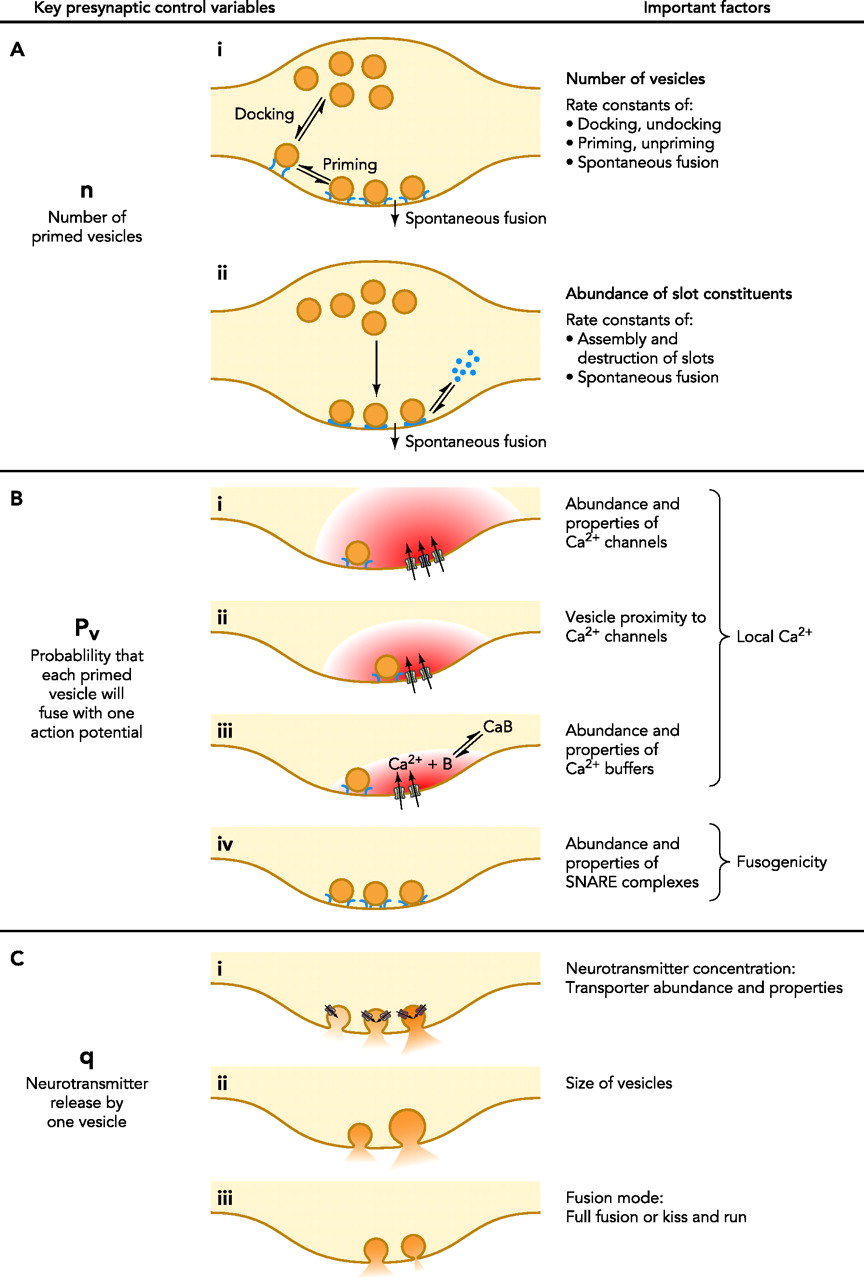Figure 3: Here are some factors that influence release of neurotransmitters from presynaptic neuron axon termini. (a) The number of primed vesicles is determined in large part by the interplay of rates of docking (and undocking), priming (and unpriming) and possibly spontaneous fusion. (b) The probability that a primed visicle will fuse with the presynaptic membrane following one action potential is largely determined by the distribution of Ca²+. SNARE proteins mediate vesicle fusion and thereby control the property of fusegenicity referred to in (iv). (c) Whether and to what degree a vesicle will release neurotransmitters into the synaptic cleft. [From Ariel and Ryan [10]]

Neurons generate two types of potential: action potentials¹⁰¹ and electrotonic potentials¹⁰². Electrotonic potentials dominate signal propagation in the soma and dendritic arbor, propagate faster than action potentials but fall off exponentially, and sum spatially and temporally by integrating input from multiple sources originating in the dendritic arbor and the cell body. Action potentials can also propagate backward toward the soma, in a process believed by some researchers to serve a similar function to backpropagation in training artificial neural networks¹⁰³.

Cortical neurons typically integrate thousands of inputs. Much of this input originates in the dendritic arbor and is combined and thresholded in the soma and axon initial segment. The axon hillock is the last site in the soma where membrane potentials propagated from synaptic inputs are summed before being transmitted to the axon. The hillock acts as a tight junction, serving as a barrier for lateral diffusion of transmembrane proteins and lipids embedded in the plasma membrane.

The axon hillock has a much higher density of voltage-gated ion channels than are found in the rest of the cell body — there are around 100-200 voltage-gated sodium channels per square micrometre compared to less than ten elsewhere in the soma. Triggering is due to positive feedback between highly crowded voltage-gated sodium channels, which are present at the critical density at the axon hillock but not in the soma.

The axon initial segment (AIS) is the site of action potential (AP) initiation. Contrary to most textbook accounts, the AIS is a complicated, special-purpose molecular machine. In most neuron types, the AIS Na+ channel density is significantly higher than at the soma and these channels are specialized for controlling AP initiation. AIS K+ channels are critical for AP repolarization and play a major role in controlling AP threshold, interspike interval and firing frequency.

The AIS includes organelles (apparently) serving the function of endoplasmic reticulum that are positioned close to the cell membrane, contain Ca²+ ion pumps, and are thought to be equivalent to structurally-similar apparatus found in dendritic spines. One obvious function of these organelles would be to sequester calcium that locally enters the AIS via voltage-gated Ca²+ ion pumps. While the AIS is not as yet fully understood, there is ample evidence to suggest that it performs non-trivial signal processing functions including temporal coding and influencing the capacity of APs initiated in the AIS to propagate (retrograde) back to the soma [145].

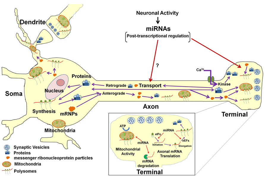Figure 4: A model for miRNA-mediated regulation of structure and function in the presynaptic nerve terminal. In the neuron, protein synthesis occurs in multiple compartments that include the cell body, dendrite, axon and presynaptic nerve terminal. A subset of mRNAs transcribed in the nucleus are packaged into stable messenger ribonucleoproteins complexes (mRNPs) and are selectively and rapidly transported to distant structural and functional domains of the neuron. The selective translation of these localized mRNAs plays key roles in neuronal development, axon growth and maintenance, and synaptic plasticity. In addition, microRNAs can also modulate translation of multiple mRNAs in the axon and nerve terminal by regulating local expression of eukaryotic translation factors (see inset). [From Kaplan et al [131]]

The distal structural and functional domains of neurons, including, of particular relevance to this log entry, the axon and presynaptic nerve terminal are the locus of an incredibly complex array of cellular machines. These include mitochondria, endoplasmic retricular structures, specialized ribosomal protein-synthesis machines called polysomes consisting of clusters of ribosomes held together by a strand of messenger RNA that each ribosome is translating, plus the terminal end of a complex cellular transport system trafficing in mRNAs, non-coding RNAs that regulate gene expression post-transctriptionally. All this machinery has significant effect on axonal protein synthesis, local energy metabolism, and the modulation of axonal outgrowth and branching [131]. See Figure 4 for more on genetic pathways.

Figure 5: Integrated model of pre- and post-synaptic myosins in cytostructural change and cellular transport. Arrows represent cellular processes that are mediated by, or are upstream of, the respective myosins. Presynaptic functions of myosins include: promotion of directed movement of synaptic vesicles (SVs) generated by endocytosis after evoked glutamate release by myosin II; and promotion of synaptic recycling of vesicles and induction of brain-derived neurotrophic factor (BDNF)-dependent long-term potentiation (LTP) by myosin VI. Postsynaptically, non-muscle myosin IIb and myosin Vb are activated by an NMDA receptor (NMDAR)-dependent Ca2+ influx. Non-muscle myosin IIb promotes the turnover of actin filaments in spines, thereby contributing to spine head growth and the maintenance of LTP. Myosin Vb trafficks AMPA receptor (AMPAR) subunit GluA1-carrying recycling endosomes (REs) into spines and thereby contributes to spine head growth and AMPAR surface delivery during LTP establishment. [From Kneussel and Wagner [139]]

Though not emphasized here, it is worth pointing out that several cytoskeletal polymers that we discussed last quarter in the context of expansion circuits are critical in maintaining the shape of spines. In particular, actin is at the crux of spine number, shape, and motility; the mechanisms that regulate actin in spines have become the topic of intense investigation. Moreover these structural polymers are highly dyanmic. Approximately 85% of actin in dendritic spines is dynamic, with an average half-life of 44 seconds independent of the size of the spines. Such rapid turnover is at odds with the concept of stable actin filaments maintaining postsynaptic components and spine integrity. See Figure 5.

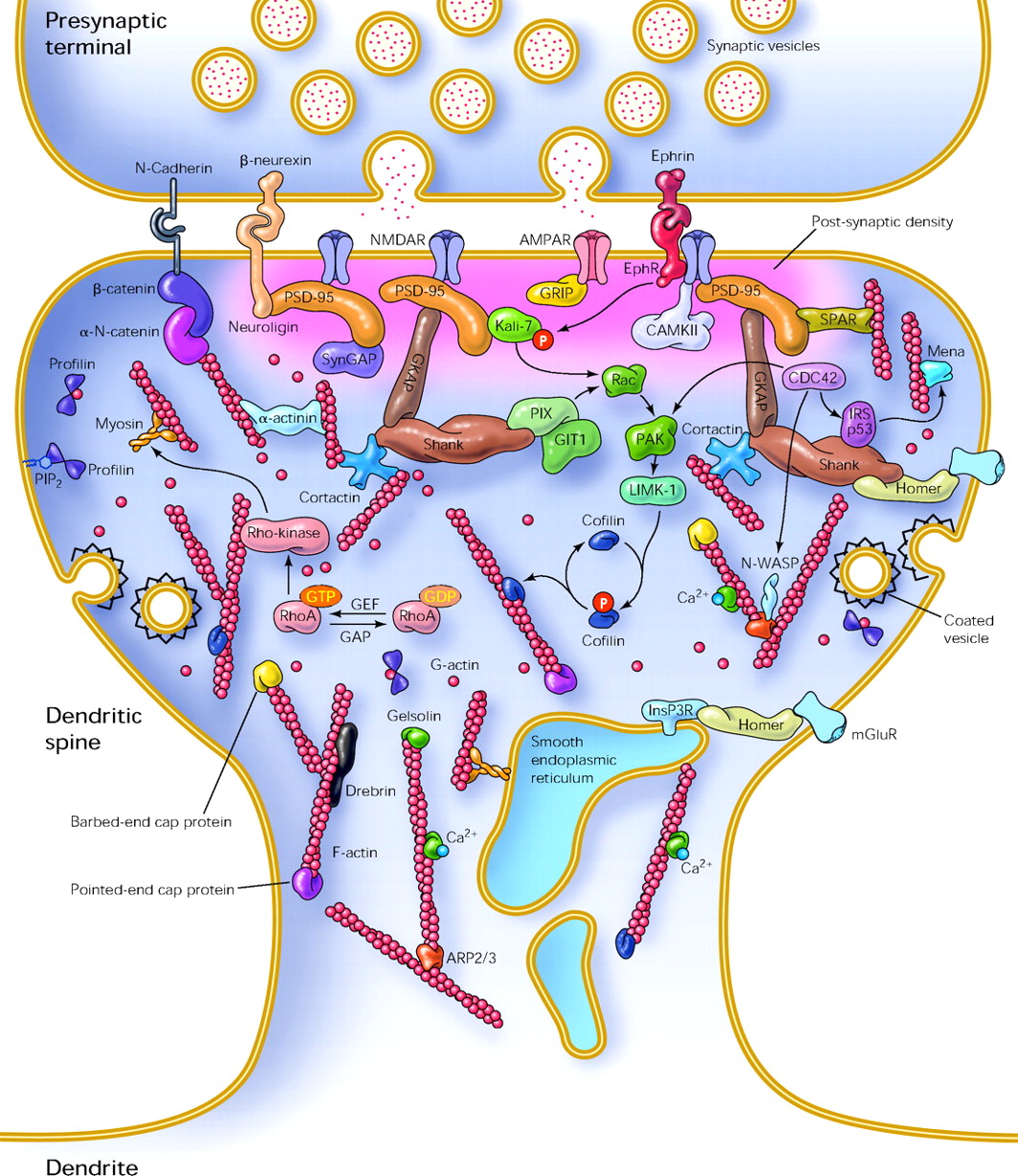Figure 6: Neurotransmitter receptors, scaffolding molecules and signaling cascades in dendritic spines. Spines are small membrane protrusions at synaptic junctions that use the excitatory neurotransmitter glutamate, which is released from synaptic vesicles clustered in the presynaptic terminal. Across from these glutamate release sites, α-amino-3-hydroxy-5-methyl-4-isoxazolepropionic acid (AMPA) and N-methyl-D-aspartate (NMDA) subtypes of glutamate receptors are clustered at the postsynaptic active zone within a dense matrix called the postsynaptic density (PSD; pink). Beyond the PSD lie subregions of spine membrane that contain G protein-coupled glutamate receptors (mGluR) and endocytic zones for recycling of membrane proteins. Receptors, in turn, connect to scaffolding molecules, such as PSD-95, which recruit signaling complexes (e.g., regulators of RhoGTPases, or protein kinases). Actin filaments provide the main structural basis for spine shape. Via a network of protein interactions, actin filaments indirectly link up with the neurotransmittter receptors and other transmembrane proteins that regulate spine shape and development, including Eph receptors, cadherins, and neuroligins. Actin-regulatory molecules such as profilin, drebrin, cofilin, and gelsolin control the extent and rate of actin polymerization. These, in turn, are regulated by signaling cascades through engagement of the transmembrane receptors. [From Calabrese et al [40]]

Dendritic spines typically receive input from a single synapse, store the strength of the synaptic connection, modify their size and shape to alter electrical properties and assist in transmitting electrical signals to the cell body¹⁰⁴. See Figure 6 for more on the molecules controlling dendritic spines.

Voltage-gated ion channels are a class of transmembrane ion channels activated by changes in electrical membrane potential near the channel. They are categorized by the type of ion transported and their function (SOURCE). Here we don't bother to distinguish "voltage-gated", "voltage-sensitive" and "voltage-dependent", and simply use "voltage-gated" as a catchall term. Perhaps the most familiar channel type is the voltage-gated sodium (Na+) channels which are responsible for the rising phase of action potentials. Voltage-gated calcium (Ca²+) channels are involved with neurotransmitter release in presynaptic nerve endings and are the basis for calcium imaging.

Potassium channels are found in most cell types and control a wide variety of cell functions. We are primarily interested here in voltage-gated potassium (K+) channels which conduct potassium ions down their electrochemical gradient, doing so both rapidly (up to the diffusion rate of K+ ions in bulk water) and selectively (excluding, most notably, sodium despite the sub-angstrom difference in ionic radius). Biologically, these channels act to set or reset the resting potential in many cells. In excitable cells, such as neurons, the delayed counterflow of potassium ions shapes the action potential. There are also voltage-gated chloride channels that open with depolarization, in a strongly pH-sensitive manner, to remove acid from cells¹⁰⁵.

The plasma membrane of neurons is complex extended molecular machine that plays a fundamental role in all facets of cellular function and, particular, its information processing activity. Only half the surface area of the membrane is covered by phospholipids. The rest consists primarily of receptor proteins, cell adhesion molecules and ion channels. The lipids and membrane proteins are organized in glycolipoprotein microdomains called lipid rafts that are more densely packed than the rest of the membrane. The spatial and temporal distribution of the membrane proteins is in constant flux adapting to suit changes in synaptic connection strength, alterations in the cytoskeletal architecture in response to changes in the size and shape of dendritic spines, and adjustments in the signaling characteristics governing action potential propagation in the axonal arbor. We briefly discussed how channel proteins control AP initiation and propagation above and will only touch on a few observations pertinent to the spike-transmission cycle. See Figure 7 for more detail on the structure and motility of dendritic spine.

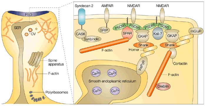Figure 7: Structure of dendritic spine showing major organelles, postsynaptic surface of synaptic cleft, etc. A mushroom-shaped spine is depicted, containing various organelles, including smooth endoplasmic reticulum (SER), which extends into the spine from SER in the dendritic shaft. SER is present in a minority of spines, correlating with spine size. The SER in spines functions, at least in part, as an intracellular calcium store from which calcium can be released in response to synaptic stimulation. In some cases, SER is seen to move close to the postsynaptic density (PSD) and synaptic membrane, perhaps by specific protein-protein interactions between PSD proteins Shank and Homer, and the inositol-1,4,5-trisphosphate receptor (InsP₃R) of the SER. Particularly common in larger spines is a structure known as the spine apparatus, an organelle characterized by stacks of SER membranes surrounded by densely staining material. The role of the spine apparatus is unknown, although it might act as a repository or a relay for membrane proteins trafficking to or from the synapse. Vesicles of 'coated' or smooth appearance are sometimes observed in spines (particularly in large spines with perforated PSDs), as are multivesicular bodies, all consistent with local membrane trafficking processes. [From Hering and Sheng [109]]

While the Hodgkin-Huxley model and its various extensions can be reasonsbly applied to macroscopic structures, e.g., the squid giant axon, they assume a lack of interaction between the local electric field and diffusional flux¹⁰⁶, an assumption that cannot be made for small neuronal microcompartments, in which electrodiffusion¹⁰⁷ is likely to be important. Moreover, local geometry at the submicron level has significant effects on the motion and distribution of charged species within the cell. Dendritic spines are morphologically complex, but can be grossly simplified as consisting of a spherical head connected by cylindrical—see Figure 8. In such submicron spaces, the variation in geometry between the two different spatial regions (head and neck) has a dramatic effect. For example,it's been shown that the decay time of the diffusion of particles (such as molecules or ions) from the spine head into the neck is dominated by diffusional coupling¹⁰⁸ between the spine neck and head.

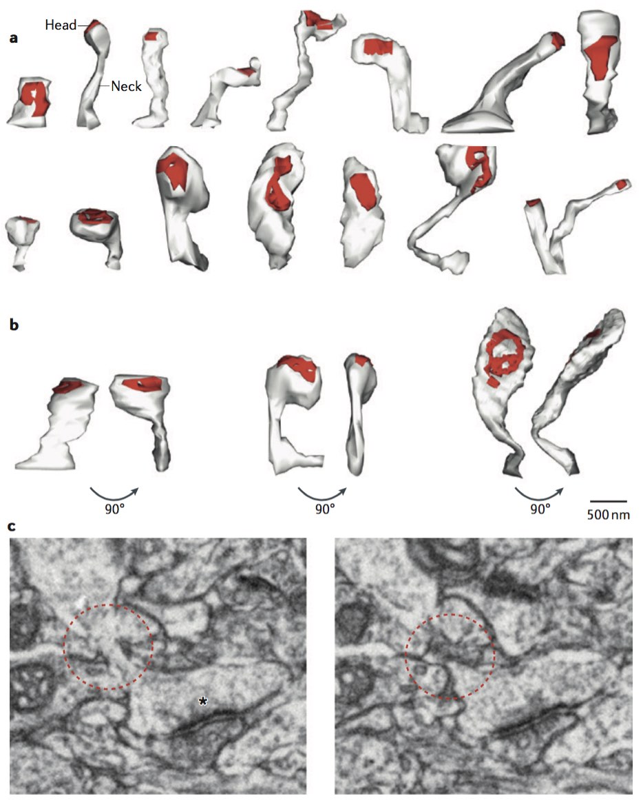Figure 8: Geometric and morphological complexity of dendritic spines illustrating head and neck features. (a) Three-dimensional ultrastructural reconstructions of spines from several layer 2/3 pyramidal cells in the mouse visual cortex. The large variability in the morphology of their heads and necks is apparent. Red areas mark the position of postsynaptic densities (PSDs). (b) Rotational views of three spines, illustrating their morphological complexity and showing how the spine neck can become physically pinched. (c) Physical obstruction of spine neck. The images show consecutive 4 nm thick serial sections cut through a dendritic spine from the mouse primary somantosensory cortex. The head of the spine is in the lower part of the images, and an asymmetric synapse can be seen (asterisk). The spine neck is open in the left section but is obstructed by an intracellular electrodense organelle in the right section (red circles). [From Holcman and Yuste [112]]

Accurately modeling electrodiffusion, diffusional coupling and related phenomena arising from the complex geometry and dynamics of neural processes is possible using more advanced computational methods like Monte Carlo simulation and more complex mathematical models like the Poisson-Nernst-Planck (PNP) equations [219]. However, this assumes you are able to acquire accurate 3D-reconstructions of the target tissue, and have good estimates for the spatial and temporal distribution of intracellular molecules that obstruct the diffusion of charged particles and extracellular molecules that induce electric fields and cause electrostatic interactions. It remains to be seen just how important this sort of nanoscale-detailed modeling is with respect to adequately understanding neural computation, but we won't know until we have gained a proper quantitative understanding of the underlying nanoscale phenomena [112]. I recommend reading the Holcman and Yuste [112] review paper as there is much to learn from the discussion. Rafael Yuste will be visiting us on Wednesday, February the 9th, and so you'll have an opportunity to ask him questions about his paper then. He'll also be giving a talk at Stanford later in the afternoon.

Figure 9: A motor neuron cell body in the spinal cord illustrating some of the many incident synapses. (a) Many thousands of nerve terminals synapse on the cell body and dendrites. These deliver signals from other parts of the organism to control the firing of action potentials along the single axon of this large cell. (b) Micrograph showing a nerve cell body and its dendrites stained with a fluorescent antibody that recognizes a cytoskeletal protein (green). Thousands of axon terminals (red) from other nerve cells (not visible) make synapses on the cell body and dendrites; they are stained with a fluorescent antibody that recognizes a protein in synaptic vesicles. [From Alberts et al[6]]

Throughout the latter part of the 20th century it was generally assumed that learning takes place in a relatively stable neural structure. I was told in an Introduction to Neuroscience course taught at Yale in 1984 that most of the neural wiring, including much of what is needed to connect pairs of neurons, is in place by the time you're twenty. I took this to mean that synapses—or at least the rough positioning of the pre- and postsynaptic neurons—was done prior to adulthood. Over the following decades new findings chipped away at this dogma and neuroscientists gradually reconciled themselves to the fact that the brain and the detailed structure of its network of neurons is highly dynamic [211, 256]. Indeed, the brain appears to change even in the absence of learning. Axons sprout and dendritic spines come and go on a time scale of days in the adult cortex—see Figure 10.

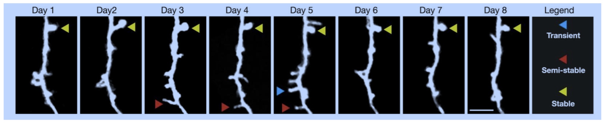Figure 10: Images of a dendritic segment exhibiting variations in spine development occurring over eight days. Examples of transient, semi-stable and stable spines (with lifetimes of less than or equal to 1 day, 2-7 days, and greater than or equal to 8 days, respectively) are indicated with blue, red and yellow arrowheads, respectively. Scale bar, 5 micrometres. [From Trachtenberg et al [256]]

In addition to synaptic transmission, there are several modes of diffuse signaling—often referred to as ectopic transmission—in mammalian and crustacean brains that can serve to alter the function of neural ensembles. Diffuse transmission is an important non-synaptic communication mode in the cerebral neocortex, in which neurotransmitters released from en passant varicosities along axons interact with surrounding cells [280]. Astrocytes, a subclass of glial cells until recently believed restricted to respiration, structural support, insulation between neurons and various housekeeping functions, now appear to actively take part in synaptic transmission and synaptic plasticity, and thereby contributing directly to neural memory formation and information processing [53].

Neuromodulation, another common mode of diffuse signaling, refers to a process whereby one or more neurons secrete substances called neuromodulators that regulate the function of diverse populations of neurons. The primary neuromodulators of the central nervous system include acetylcholine, adenosine, dopamine, Gamma-Aminobutyric acid, histamine, norepinephrine and serotonin, all substances that serve multiple roles in the nervous system. Neuromodulators secreted by a small group of neurons propagate by diffusion through the cerebrospinal fluid, affecting multiple neurons, but with less precision than syntactic transmission. Neuromodulation can switch the function individual neurons and small neural circuits to perform different computations depending on the ambient environment [13, 164].

Figure 11: Reversal potentials and threshold potentials determine excitation and inhibition. The reversal potential (E_rev) is the membrane potential of a post-synaptic neuron (or other target cell) at which the action of a given neurotransmitter causes no net current flow (SOURCE). (a) If the reversal potential for a PSP (0 mV) is more positive than the action potential threshold (-40 mV), the effect of a transmitter is excitatory, and it generates EPSPs. (b) If the reversal potential for a PSP is more negative than the action potential threshold, the transmitter is inhibitory and generate IPSPs. (c) IPSPs can nonetheless depolarize the postsynaptic cell if their reversal potential is between the resting potential and the action potential threshold. (d) The general rule of postsynaptic action is: If the reversal potential is more positive than threshold, excitation results; inhibition occurs if the reversal potential is more negative than threshold. [From Purves et al [56]]

Molecular tagging and drug delivery protocols typically involve engineering diffusion-reaction processes in which molecular payloads intermingle with the molecules of a tissue sample in solution at a rate that depends on their kinetic energy due to random motion and several other factors. Diffusion in the extracellular space (ECS) of the brain is constrained by the composition of the interstitial fluid, the ECS volume fraction — approximately 20% in normal brain tissue — and its tortuosity¹⁰⁹.

Given values for these parameters a modified diffusion equation can approximately predict the transport behavior of many molecules in the brain. However, to achieve more accurate predictions, you'll need to account for the loss of molecules across the blood-brain barrier, through cellular uptake, binding or other mechanisms as well geometric constraints including spaces that inaccessible space due to constrictions and the size of the molecular payload.

Recent work on expansion circuits relies heavily on such reaction diffusion-processes to facilitate molecular self-assembly. The task of installing nanoscale computing elements is made somewhat more tractable by the fact that we can expand the tissue and eliminate a substantial fraction of the molecular clutter to allow passage of large payloads on the order of 100 μm on a side. The images in Figure 12 illustrate the composition of neural tissue and the matrix in which diffuse signaling must function.

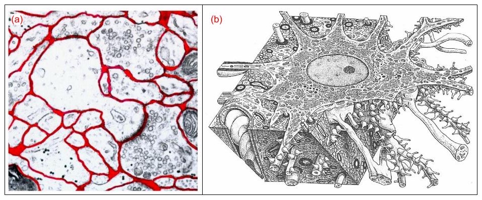Figure 12: An electron-micrograph and an anatomical drawing illustrating the dense composition of neural tissue. (a) Electron-micrograph of small region of rat cortex with dendritic spine and synapse. The ECS is outlined in red; it has a well-connected foam-like structure formed from the interstices of simple convex cell surfaces. Even though the ECS is probably reduced in width due to fixation procedure it is still evident that it is not completely uniform in width. Calibration bar approximately 1 μ. (b) An illustration from an anatomy textbook depicting the molecular clutter of both intra- and extracellular space along with a pretty reasonable artistic rendering of the spatial distribution of axosomatic and axodendritic synapses. [From (a) Sykova and Nicholson [253] and (a) Fletcher [77]]

The neuronal membrane gets much less attention than it deserves. The fact that cable theory models the membrane as an assembly of 1D compartments underscores this neglect. A typical neuron has thousands of synapses. Some tend to excite the neuron resulting in an excitatory postsynaptic potential (PSP) and causing a small depolarization of the membrane, and some synapses tend to inhibit the neuron resulting in an inhibitory PSP causing a hyperpolarization of the membrane. Inhibitory neurotransmitters open either Cl- channels or K+ channels, making it harder for excitatory influences to depolarize the postsynaptic membrane—see Figure 11.

Synapses in the same neighborhood approximately sum with the inhibitory PSPs making a negative contribution, and then passively spread out propagating in all directions in the dendritic tree, eventually converging on the cell body. The propagating wave fronts are exponentially attenuated as they move toward the soma. In the standard account taught in most neuroscience courses [6], the dendritic conduits are assumed to have no interesting shape or internal structure, and the computational story is relatively simple:

Because the cell body is small compared with the dendritic tree, its membrane potential is roughly uniform and is a composite of the effects of all the signals impinging on the cell, weighted according to the distances of the synapses from the cell body. The combined PSP of the cell body thus represents a spatial summation of all the stimuli being received. If excitatory inputs predominate, the combined PSP is a depolarization; if inhibitory inputs predominate, it is usually a hyperpolarization.
Whereas spatial summation combines the effects of signals received at different sites on the membrane, temporal summation combines the effects of signals received at different times. If an action potential arrives at a synapse and triggers neurotransmitter release before a previous PSP at the synapse has decayed completely, the second PSP adds to the remaining tail of the first. If many action potentials arrive in quick succession, each PSP adds to the tail of the preceding PSP, building up to a large sustained average PSP whose magnitude reflects the rate of firing of the presynaptic neuron. This is the essence of temporal summation: it translates the frequency of incoming signals into the magnitude of a net PSP. [From Alberts et al[6]]

Clearly this is a fictional account if we are to believe Holcman and Yuste [112]. The question is whether this or some other equally simple story provides an adequate foundation on which to build a comprehensive computational theory of neural function. Is the Alberts et al[6] account a Newtonian theory sufficient as a basis for predicting planetary motions, to be supplanted in time by a more comprehensive relativistic model? Or is it Copernican and of little practical use, or Ptolemaic and seriously misleading. This may seem like a silly question, but I suggest that we don't know enough to definitively say one way or the other.

Mark Ellisman, Terry Sejnowski, Steven Smith and now Ed Boyden have seemingly retreated from trying to solve the larger problem of reducing behavior to computation. Instead they are digging in for a long campaign, admitting there is too much we don't know, and resigning themselves to the long and arduous task of identifying, measuring, recording, quantifying and categorizing every molecule and reaction they can in the hope that a clear story will emerge. I'm too impatient to make that commitment, and I don't need a molecular-scale account of neural function if my goal is to leverage biological insight in order to build a better robot vision system.

I want to devise experiments that will enable me to crack open the door just wide enough to admit a slender ray of light that suggests an algorithmic principle or reveals a mathematical intuition I can use to deliver better, faster, more efficient computational solutions. The problem with the likes of Ibn al-Shatir, Nicolaus Copernicus, Johannes Kepler and Tycho Brahe wasn't that they couldn't fit the data — their models were so flexible they could fit most any data — the problem was that they couldn't predict anything beyond the data.

January 11, 2016

I met with Dmitri Strukov from UC Santa Barbara on Tuesday morning. For several years before setting up his own lab at UCSB, Dmitri worked at HP Labs with Stan Williams and the team that developed the Titanium Oxide memristor. I was already familiar with most of the research from Dmitri's lab that was featured in his talk, but I learned a lot about failures, experimental details and technical challenges that don't end up in academic papers. I also learned about some of the companies besides HP pursuing memristor technology. What is now called resistive random-access memory — basically memristors without the neuromorphic baggage — is being pursued by several flash memory companies—see Rambus. Hafnium Oxide has emerged as the dielectric of choice, dethroning the Titanium Oxide technology that Hewlett-Packard developed and championed prior to abandoning their strategy of making memristors the linchpin of their next-generation computing effort.

I learned more about the problem of runaway instability in spiking neural networks implemented as analog circuits, the consequences of analog arithmetic in convolutional networks, and how manufacturing variability makes it difficult to mass produce consumer electronics with memristor technologies—training one model and then burning the resulting coefficients into each chip doesn't work when all the memory elements behave slightly different. Dmitri mentioned that the simulations developed in the EPFL Blue Brain and EU Human Brain Projects run 10,000 times slower than real-time on an IBM (Blue Gene) supercomputer, providing motivation for hardware simulation. I got a better understanding of the physics governing how different memristor technologies work, the implications for fabrication and large-scale manufacture, and the various interconnect technologies—see Crossbar. We agreed that 3D deposition printing of memristor devices should be significantly easier than printing conventional, e.g., CMOS, transistors. It actually is possible to print memristors now, but 3D printing technology has a long way to go before this can be done reliably and at scale.

January 9, 2016

I took a step back last week and spent some time thinking about what some of the best neuroscientists in the field are working on and whether Google might find it interesting enough to invest in. I'm not planning to suggest that Google start funding neuroscientists. Rather, I thought the exercise might help me to think about projects that would make sense for Google and, in particular, Neuromancer to pursue. All of the scientists I selected fell into multiple categories. For this exercise, however, I assigned them to just one and not necessarily the category that they or their peers might have selected. Here is my list of twenty scientists, sorted into five categories:

Ed Boyden, Winfried Denk, Michael Dickinson, Mark Schnitzer — instrument builders ...
Davi Bock, Clay Reid, Sebastian Seung, Stephen Smith — experimental neuroscientists ...
Mark Bear, Karl Deisseroth, John Donoghue, Helen Mayberg — therapeutically motivated ...
Surya Ganguli, Nancy Kopell, Konrad Kording, Bruno Olshausen — theoretical neuroscientists ...
Eugene Izhikevich, Eve Marder, Henry Markram, Terry Sejnowski — model builders ...

I'm not going to transcribe my notes and reveal how I'd parcel out funding if any. I will say that I wouldn't put any of them in charge of a project at Google, and I'm pretty sure they wouldn't want to lead a Google project. What I found most useful was thinking about how they select projects and apportion effort in their labs in terms of level of difficulty, expectation of success, tolerance for failure, relevance to socially or scientifically anointed goals, and time to return on investment.

Personally my inclination is to work on problems and apply methods that are outside of the mainstream. I agree with Brian Arthur and Matt Ridley that science and technology are evolutionary processes and that, more often than not, the latter leads the former in terms inventing the future. Scientists generally aren't the drivers of innovation; as a group they tend to be more cautious than they like to let on.

Entrepreneurs may be more willing to take risks because the financial stakes are higher. Both scientists and engineers are somewhat at a disadvantage in that their sources of approbation, funding and venture capital tend to be conservative and disinclined to support projects they consider unfamiliar or unpopular. Which is too bad given that popular and familiar projects are the most likely to be solved by multiple parties whether or not they receive support. In short, they're inevitable and not terribly lucrative investments.

I favor the unpopular and unfamiliar because they have the best chance of leading to new and unexpected advances in science and technology, and, if tackled with the right mindset, the most likely to yield value even if they don't solve the problem they set out to solve. The right mindset involves working on the hardest parts first, learning from failure, exploiting serendipity, and stepping aside and letting the engineers at it once there is a clear solution path. Easy to say and hard to do.

So, if the unpopular and unfamiliar won't motivate investors to fight for equity in your project, how do you sell it? Demonstrate that, contrary to received wisdom, there really are pieces of the puzzle already in place. Identify some initial experiments that can be carried out with existing technologies to reveal the hidden promise. Make it clear there are others who share your enthusiasm for seemingly isolated parts of the problem and that you can channel their efforts to accelerate development. So in that spirit:

Why not follow the likes of Eugene Izhikevich, Henry Markram, etc., and harness existing technologies to simulate an entire brain? It'd big and bold to be sure. It'd also inevitable given the incremental path, but also years and billions of dollars in the future. Why not follow Kwabena Boahem, Dharmendra Modha, Peter van der Made, etc., and work on something simpler and smaller scale, say, neuromorphic computing? If it was that easy, someone would have demonstrated success on some problem of interest and made millions.

We know a lot of "stuff", but we're not at all clear we have learned anything we can take to the bank as yet. One thing clear is that we've barely scratched the surface of what there is to know. As a consequence, the lack of experimental data is driving the likes of Boyden, Schnitzer, Vaziri and others to follow in the footsteps of Stephen Smith and Mark Ellisman, i.e., build new technology to record everything and then sort it out later ... necessary, but smacks of stamp collecting ... grinding microscope lenses ... etc.

Hodgkin-Huxley's model for action potentials in giant squid axons was an accomplishment worthy of a Nobel Prize, but let's face it, their model was a special case of the theory that William Thompson (Lord Kelvin) and Oliver Heaviside developed in the 1900s to account for signal attenuation in transatlantic telegraph cables. The same goes for early work on the crustacean stomatogastric ganglion—a simple model for a simple organism but hard to generalize to mammal cortical circuits. Electron microscopes are wonderful tools but it was semiconductor fabrication and materials engineering that drove their refinement.

Relative to my enthusiasm for large-scale simulation, what impact can we expect from a 100-times faster NEURON or MCELL. There's good science to be done, but we still don't know enough to build accurate models and learning how will take time ... perhaps a lot of time. Waiting may be the best strategy since it's likely Moore's law will do its accelerating-returns magic trick and outpace legions of bench scientists in short order ... shades of the textile workers in the first industrial revolution ... enchanted looms be damned.

As my next exercise, I plan to do a survey of what we know — and don't know — about spiking neurons that would improve our ability to model the behavior of reasonably sized — millions of neurons — ensembles. I also want to review work from Harvard on a neuromorphic synaptic transistor capable of spike-timing-dependent plasticity learning [229] and recount my recent conversation Dmitri Strukov [202, 276, 249].

January 7, 2016

In most areas of neuroscience—excluding some flavors of theoretical and computational neuroscience, the term function is generally not intended to invoke the idea of computing a mathematical function. More often than not, the word and its variants are used to represent relationships between physiological markers that may or may not facilitate computation¹¹⁰.

Hypotheses concerning capabilities, e.g., in terms of proteins expressed and neurotransmitters released, abound. Examples of how these capabilities give rise to specific computations are far less common. Roth and van Rossum [212] offer plenty of the former, Larry Abbott and his colleagues have done a pretty good job in summarizing some of the latter [2, 1].

I've consolidated and extracted what I consider to be the most relevant excerpts from the Abbott and Regehr paper below. I've also included a selection of references and linked papers that were cited in the Abbott paper and that I found particularly relevant to our discussion of computational primitives¹¹³. If you read only one paper cited in this log entry, I recommend the 2004 paper by Abbott and Regehr appearing in Nature (PDF).

AN EXPLANATION AND DISCLAIMER CONCERNING THE SEMICONDUCTOR ANALOGY FOR SYNAPSES

A synapse is more than an assembly of the molecules that comprise the synaptic cleft and its immediate environment. Any computational account of a synapse necessarily involves neighboring mitochondria and endoplastic reticulum, the distant soma and related cellular transport machinery, and a host of chemical, electrical and genomic pathways.

Despite my earlier analogy, transistors are not like synapses. Transistors happen to be more complicated than most people think—including a lot of engineers, and hence their value as a bridging analogy, but we have engineered electronic components to be extraordinarily well behaved in order to facilitate abstractions simplifying the design of electronic circuits.

The advantage of these abstractions is that we don't have to account for all the complex physics that make transistors work. Electrical engineers rarely think in terms of electrons, holes, quantum tunneling, etc., when designing electronic circuits. The quantities voltage, current, resistance, etc., along with Kirchhoff's current and voltage laws suffice for most designs.

Neural circuits aren't so accommodating, we have to account for more than just spike trains and local field potentials. The distribution of neurotransmitters, expressed proteins, voltage-gated ion channels, calcium concentrations, etc. are part of the information state vector of a synapse, and figure in its immediate and future activity.

To isolate and abstract the function of a synapse in a neural circuit, we would need to know what information is transmitted to the postsynaptic neuron (feedforward) and understand what the presynaptic neuron receives in return (feedback). In principle, we could encode all of the electrical, chemical and proteomic signals as a binary vector.

To learn a synaptic model from recorded data, however, we'd have to convert (translate) observable events, e.g., calcium imaging rasters, vesicle counts, etc., into vectors that capture this information. Suppose we model synapses as artificial neural networks. What sort of vectors would we need to generate to reproduce the synaptic behavior?

The hard part involves coming up with concise abstraction for the I/O; nature is not as accommodating as Intel in providing compact, complete and comprehensible abstractions; the spike train only tells part of the story, there is much more information packed away in the adjacent neurons, the structural proteins that connect them, etc.

SYNAPTIC PLASTICITY: MECHANISMS GOVERNING ACTIVITY-DEPENDENT CHANGES IN TRANSMISSION

Activity-dependent changes in synaptic transmission arise from a large number of mechanisms known collectively as synaptic plasticity. Synaptic plasticity can be divided into three broad categories: (1) long-term plasticity, involving changes that last for hours or longer, is thought to underpin learning and memory; (2) homeostatic plasticity of both synapses and neurons allows neural circuits to maintain appropriate levels of excitability and connectivity despite changes brought about by protein turnover and experience-dependent plasticity; (3) short-term plasticity, which is the main focus of this review, occurs over milliseconds to minutes and allows synapses to perform critical computational functions in neural circuits.

COMPUTATIONS ARISING FROM SHORT-TERM—MILLISECONDS TO MINUTES—SYNTACTIC TRANSMISSION

On rapid timescales (milliseconds to minutes) the release of neurotransmitter depends on the pattern of presynaptic activity, and synapses can be thought of as filters with distinctive properties. This provides synapses with computational potential and has important implications for the diversity of signalling within neural circuits. Neural responses are typically described by specifying the sequences of action potentials that neurons fire.

So, each neuron transmits not just one, but a large number of different signals to the neural circuit in which it operates. Individually, these synapse-specific signals are selectively filtered versions of the action potential sequence that the neuron generates, modified by the context of previous presynaptic and postsynaptic activity. Collectively, knowing which synapses transmit a given action potential— the signal by which neurons interact — provides more information than simply knowing that a neuron has fired. Communication from a single neuron is thus a chorus not a single voice.

FORMS OF SYNAPTIC PLASTICITY: INCLUDING MECHANISMS FOR BOTH FEEDFORWARD AND FEEDBACK

Several forms of plasticity are feedforward in character, meaning that their induction depends solely on presynaptic activity. Such forms of plasticity are the main focus of this review. However, the flow of information across a synapse can also be bidirectional, which greatly enhances computational potential. Synaptic plasticity can depend on feedback from the postsynaptic neuron through the release of retrograde messengers. This feedback plasticity may operate in isolation or in conjunction with presynaptic activity (associative plasticity). Feedforward, feedback and associated forms of synaptic plasticity have quite different functional and computational implications.

The type of receptor activated at the synapse also affects the postsynaptic response. Glutamate, for example, can activate AMPA receptors, NMDA receptors, and metabotropic glutamate receptors (mGluRs). AMPA receptors show a range of properties but usually have rapid kinetics. NMDA receptors have much slower kinetics and are voltage dependent. mGluRs are coupled to second messenger systems that can lead to modulation and activation of channels and to the release of calcium from internal stores. Finally, the location of a synapse on the dendritic arbor in relation to the general morphology of the neuron and its distribution of active conductances, as well as the presence of other active synapses, all have important roles in determining the postsynaptic response.

Numerous mechanisms of plasticity acting over a wide range of timescales influence the release of neurotransmitter-containing vesicles. The initial probability of release and use-dependent plasticity of synapses are determined by the identities of the presynaptic and postsynaptic neurons, as well as by the history of action potential activity and by the local environment. There are numerous examples of boutons from the same axon giving rise to facilitating synapses (that enhance synaptic strength) for some types of target neurons and to depressing synapses (that reduce synaptic strength) at others.

FEEDFORWARD FACILITATION AND DEPRESSION GOVERNS PROBABILITY OF NEUROTRANSMITTER RELEASE

Periods of elevated presynaptic activity can cause either an increase or a decrease in neurotransmitter release. Facilitation reflects an increase in the probability of neurotransmitter release (p) that lasts for up to hundreds of milliseconds. Depression reflects a decrease in the probability of neurotransmitter release that persists for hundreds of milliseconds to seconds. Facilitation and depression seem to coexist at synapses, with their relative weight depending largely on the initial p: high p favours depression, low p favours facilitation.

FEEDBACK PLASTICITY MEDIATED BY RETROGRADE MESSENGERS REGULATE NEUROTRANSMITTER RELEASE

Recent studies have also identified plasticity operating on rapid timescales that depends on postsynaptic activity. Several retrograde messengers have been identified that once released from dendrites act on presynaptic terminals to regulate the release of neurotransmitter. The endocannabinoid system is the most widespread signalling system that mediates retrograde signalling. [...] This release of endocannabinoids leads to an inhibition of neurotransmitter release that lasts for tens of seconds. [...] This suggests that the state of the postsynaptic cell exerts control on neurotransmitter release from the presynaptic terminals by regulating the release of endocannabinoids.

ASSOCIATIVE PLASTICITY ON SECONDS TO TENS-OF-SECONDS TIMESCALE COULD SERVE BACKPROPAGATION

Short-term forms of associative plasticity would be useful for several reasons. Network models based on short-term plasticity can lead to persistent activity in a subset of neurons that represent a particular memory. Models based on fast associative plasticity are more robust than models relying solely on finely tuned synaptic weights within the network. Rapid associative plasticity could also be useful for improving performance on a task where predictions are made and then error signals are used to correct deviations from those predictions. This is because associative plasticity allows the error signal to make appropriate corrections by modifying synapses that lead to incorrect performance.

FUNCTIONAL ROLES OF SHORT TERM PLASTICITY IN CONTROLLING SIGNAL FACILITATION AND DEPRESSION

Short-term synaptic plasticity can drastically alter how a neuron activates its postsynaptic targets. [...] The climbing fibre synapse has a high initial p and therefore depression dominates the short-term plasticity during bursts, with gaps in the presynaptic activity allowing recovery. Parallel fibre synapses are low p synapses and facilitation dominates their short-term plasticity, with relaxation occurring during pauses in presynaptic activity. Hippocampal Schaffer collateral synapses have an intermediate p and show a large transient enhancement of synaptic strength but a less pronounced steady-state level of enhancement.

ADAPTIVE CONTROL OF SYNAPTIC FILTERING SHAPING FREQUENCY MODULATED SIGNAL PROPAGATION

An important consequence of synaptic dynamics is that synapses can act as filters with a wide range of properties. Synapses with a low initial probability of neurotransmitter release, such as parallel fibre synapses, function as high-pass filters, whereas synapses with a high initial probability of release, such as climbing fibre synapses, act as low-pass filters that are most effective at the onset of presynaptic activity. Synapses with an intermediate probability of release, such as Schaffer collateral synapses, act as band-pass filters that are most effective at transmitting impulses when there is an intermediate range of presynaptic activity.

The filtering characteristics of a given synapse are not fixed; they can be adjusted through modulation of the initial release probability or other aspects of synaptic transmission. Many neuromodulators activate presynaptic receptors, and the result is often a reduction in the probability of release. As a result of this decrease in the amount of neurotransmitter released, the filtering characteristics of the modulated synapse are altered so that depression makes a smaller contribution to synaptic dynamics and facilitation becomes more prominent. In this way, presynaptic inhibition can convert a synapse from a low-pass filter to a band-pass filter, or from a band-pass filter to a high-pass filter.

CONTRAST ADAPTATION AND THE ENHANCEMENT OF TRANSIENTS IN RESPONDING TO NOVEL STIMULI

Neurons typically respond most vigorously to new rather than to static stimuli. Synaptic depression provides a possible explanation for this virtually universal feature of sensory processing. Consider the case of sensory input to a neuron A that in turn excites neuron B through a depressing synapse. Even if a prolonged sensory stimulus activates neuron A in a sustained manner, the response of neuron B may only be prominent at the onset of stimulation because synaptic depression produces a synapse-specific decrease in the drive to neuron B. This results in a neuron that only responds to new stimuli. Synaptic depression acting in this manner may contribute to contrast adaptation and to suppression by masking stimuli in primary visual cortex.

FLOW OF INFORMATION BETWEEN PRE AND POST-SYNAPTIC NEURONS INCLUDES STATE INFORMATION

Transmission across a synapse is obviously the conveyance of information carried in a presynaptic action potential to the postsynaptic neuron. However, for dynamic synapses each synaptic transmission also contains information about the previous history of spiking. This contextual information can be quantified. Synaptic plasticity assures that current activity reflects both the current state of a stimulus and the previous history of activity within the neural circuit.

SYNCHRONIZATION, TIMING AND RATE CODING FOR SOUND LOCALIZATION AND BINAURAL HEARING

Synaptic depression may also have an important role in sound localization. In the avian brain, neurons in nucleus laminaris (NL) represent the spatial location of a sound. Firing of NL neurons requires precisely coincidental arrival of binaural input, and results in high sensitivity to differences in sound conduction delays between the two ears, and so to sound location. These neurons localize sounds over a broad range of intensities. Increases in sound level elevate the firing rates of the inputs to NL neurons, suggesting that intensity could be a complicating factor in spatial discrimination.

DYNAMIC INPUT COMPRESSION AND SCALING TO ACCOMMODATE LARGE CHANGES IN ILLUMINATION, ETC

Neurons integrate thousands of inputs, each firing over a range of about 1-100 Hz. But they keep their output firing rates within this same range. Doing this requires precise mechanisms of gain control and input compression. Sensory systems face similar compression problems owing to the enormous range of intensities found in nature for most stimuli. Many sensory responses obey a Weber-Fechner law, meaning that changes in stimulus intensity are interpreted in relative or percentage terms rather than on an absolute scale. This results in a logarithmic compression of the intensity scale. Synaptic depression seems to allow a similar form of compression to occur at the neuronal level. This is because, when depression is occurring, the level of synaptic transmission at high rates is proportional to the inverse of the presynaptic firing rate. A rapid change in the presynaptic firing rate thus results in a transient synaptic current that is proportional to the size of that change scaled by the baseline firing rate.

January 5, 2016

I think there's an insight buried in this note, but I've struggled to make it clear and so far been disappointed with my efforts. If forced to summarize my argument at this stage, I'd say something like the following:

Synapses are not arbitrary functions. They are limited in function to a small number of computational primitives. In this respect, they are analogous to transistors in electronic circuits that can be categorized as serving as amplifiers or switches. If we can identify the class of synaptic primitives, we can simplify fitting models to reproduce neural circuit behavior. In this view, reconstructed neural circuitry is the primary source of computational novelty that we can expect to infer from neural tissue.

In this log entry, we consider the factors driving the evolution of computation in biological organisms, contrasting these factors with those driving the commercial development of computer technology. To make our central points, we focus on semiconductor technology from the late 1940s to the present and compare with recent progress in neuroscience studying the diversity of synapses [33, 48, 279, 74, 100, 151, 173, 102]. We argue that synapses perform the functions of a small set of computational primitives, that the apparent diversity of synapses found in nature reflects a specialization of function, an accommodation in manufacture, or an artifact of natural selection's conservative iterative-design process.

The variability we observe in nature is analogous to what one might expect if a transistor design was copied by several manufacturers, each one making small alterations to meet the operating characteristics required of their customer's product line. An engineer designing a prototype, could use any one of several transistors from different suppliers in a given circuit as long the device chosen satisfies the circuit requirements in terms of size, power, forward and reverse beta, frequency response, etc. We start by examining the sources of variability in semiconductor devices to demonstrate that while there is diversity in their specifications, transistors have a limited computational repertoire. If the same is true of synapses, we will have an easier time imposing an appropriate selection bias to constrain search in modeling neural circuits.

Bipolar junction transistors (BJTs) are current controlled while field effect transistors (FETs) are voltage controlled leading to different operating characteristics making them suitable for different applications. Generally speaking, BJTs are common in amplifier circuits and FETs are common in digital circuits (MOSFET) though each has wider application and there are hybrid circuits that combine BJTs and FETs to exploit their different characteristics.

Contrary to the simple treatment presented here¹¹⁴, comparing BJT and FET technologies is considerably complicated by the fact that there are many variations on each type of transistor. Innovation in transistor design was robust even before the AT&T announcement in 1951 and more so in the years immediately following. The economic incentives have only increased with new products and rapidly expanding markets. Today there are easily hundreds of types of transistor differentiated by their composition, size, 3D geometry, method of fabrication and governing physical principles.

BJTs and FETs rely on different physical principles, QFETs exploit quantum-tunneling to increase switching speed and there are many other types of FET as well as variations of the BJT design. Size matters; as transistors and interconnects shrink below 10 nanometers, different physical principles apply, requiring innovations in lithography and forcing engineers to devise novel methods for moving information within circuits, e.g., using photonics, and exploring new architectures utilizing in-place algorithms where data and computing are co-located.

Different transistor technologies employ different composition substrates including elemental, e.g., Silicon and Germanium, and compound, e.g., Gallium Nitride, Gallium Arsenide and Silicon Carbide, substrates, as well as different impurities, e.g., creating N-type semiconductors by doping silicon with other elements having five valence electrons such as Antimony, Arsenic and Phosphorous to increase the free electrons, or creating P-type semiconductors with elements having three valence electron such as Boron, Gallium and Indium to Silicon to create a deficiency of electrons or hole.

Multi-gate (MuG), ultra thin body (UTB) transistors, e.g., FlexFETs and FinFETs, using silicon-on-insulator (SOI) substrates are the current favorite in the race to sustain Moore's law, but there are other technologies in competition. Carbon, long considered to be an unlikely basis for semiconductor fabrication, is now in the running as scientists and engineers explore the properties of carbon nanotubes and buckyballs—the latter named after Buckminster Fuller.

With free-market economics powered by entrepreneurial scientists and engineers supplying the selection pressure, transistors have evolved from the first commercial devices measuring a centimeter in length and barely functional by modern standards to entire computers comprised of billions of transistors on a chip less than a centimeter in diameter and thousands of specialized devices enabling an incredible array of products that boggles the mind. All of this playing out in little more than half a century. How long is the natural-world analog of an Intel tick-tock cycle?

There are some operations biological organisms have to perform that natural selection has seen fit to conserve over millions of years and across a wide range of species. Certainly the method of encoding genotypes for subsequent reproduction using DNA and RNA is one such operation. It also stands to reason that the operations involved in communication and computation, while varied in their implementation, are highly conserved in terms of their basic function.

What are those basic functions? In a digital computer, the Boolean operators constitute a basis for all computations including both logical and arithmetical. In an analog computer, the basic operators consist of amplifiers, integrators, inverters and multipliers that might be implemented with hydraulic components such as pumps, pipes, reservoirs and valves, mechanical components such as servos, cams and gears, or electrical components such as resistors, capacitors and operational amplifiers.

The point of this exercise is to suggest that the diversity of synapses and signal pathways found in brains might be functionally less diverse than imagined. While there are many different types of transistors they are all basically amplifiers or switches with varying operating characteristics. They can be assembled into circuits that can perform a much wider range of function, including multi-stage amplifiers, timers, oscillators, analog and digital computers. Complexity doesn't arise at the level of the individual synapse, ion channel, etc., but rather at the circuit level which may have its own primitives in the form of recurring motifs that would serve to further restrict the space of neural circuit models.

Certainly the analogy doesn't apply to the extent that if one wire is out of place or one transistor fails your ALU will be useless to an accountant. Clearly the brain is more robust in some ways than a silicon chip. If the data we collect from calcium imaging is sufficient to discriminate between synaptic computational primitives—which, it won't have escaped your attention, we have yet to enumerate, and the EM data allows us to reconstruct the 3D geometry of neural circuits including structural characteristics that constrain compartmental transfer functions¹¹⁵, then I believe we may have a good chance of modeling and emulating the behavior of such circuits.

Miscellaneous loose ends: Are long term memories stored in the extracellular matrix? Terry Sejnowski at UCSD and the Salk Institute thinks so (PDF), and Sakina Palida, a graduate student working in Roger Tsien's lab at UCSD has some preliminary evidence supporting this hypothesis (PDF). Also see recent news about Janelia's drosophila optic lobe dataset and this teaching note about insect brains.

January 3, 2016

Spent the last couple of weeks reviewing organic chemistry and solid-state physics relevant to different facets of the projects I'm developing at Google as well as to the likely topic of CS379C this Spring. Sunday I collected a basic set of concepts and definitions in one place to serve as a quick review and handy reference for the students taking the class, most of whom will be in either Computer Science or Electrical Engineering. To begin with, I made a list of the forces that have to be accounted for—at least to some degree—in predicting the consequences of reaction-diffusion processes whether you're interested in neurons or semiconductors:

Coulomb's inverse-square law is a law of physics describing the electrostatic interaction between electrically charged particles. The law was essential to the development of the theory of electromagnetism and is analogous to Isaac Newton's inverse-square law of universal gravitation. Coulomb's law holds even within atoms, correctly describing the force between the positively charged atomic nucleus and each of the negatively charged electrons. This simple law also correctly accounts for the forces that bind atoms together to form molecules and for the forces that bind atoms and molecules together to form solids and liquids. Generally, as the distance between ions increases, the energy of attraction approaches zero and ionic bonding is less favorable. As the magnitude of opposing charges increases, energy increases and ionic bonding is more favorable. (SOURCE)
Van der Waals forces, named after Dutch scientist Johannes Diderik van der Waals, are the residual attractive or repulsive forces between molecules or atomic groups that do not arise from a covalent bond or electrostatic interaction. The resulting van der Waals forces can be attractive or repulsive. Van der Waals forces include attraction and repulsions between atoms, molecules, and surfaces, as well as other intermolecular forces. They differ from covalent and ionic bonding in that they are caused by correlations in the fluctuating polarizations of nearby particles as a consequence of quantum dynamics. Intermolecular forces have four major contributions (SOURCE):
1. A repulsive component resulting from the Pauli exclusion principle that prevents the collapse of molecules.
2. Induction—also known as polarization—which is the attractive interaction between a permanent multipole on one molecule with an induced multipole on another.
3. Dispersion which is the attractive interaction between any pair of molecules, including non-polar atoms, arising from the interactions of instantaneous multipoles.
4. Attractive or repulsive electrostatic interactions between permanent charges (in the case of molecular ions), dipoles (in the case of molecules without inversion center), quadrupoles (all molecules with symmetry lower than cubic), and in general between permanent multipoles.
Brownian motion is the random motion of particles suspended in a fluid (a liquid or a gas) resulting from their collision with the quick atoms or molecules in the gas or liquid. Atoms and molecules had long been theorized as the constituents of matter, and many decades later, Albert Einstein published a paper in 1905 that explained in precise detail how the motion that the botanist Robert Brown had first observed through his microscope in 1827 was a result of the pollen being moved by individual water molecules¹¹⁶. This explanation of Brownian motion served as definitive confirmation that atoms and molecules actually exist. The direction of the force of atomic bombardment is constantly changing, and at different times the particle is hit more on one side than another, leading to the seemingly random nature of the motion. Brownian motion is among the simplest of the continuous-time stochastic processes, and it is a limit of both simpler and more complicated stochastic processes. This universality is closely related to the universality of the normal distribution. In both cases, it is often mathematical convenience, rather than the accuracy of the models, that motivates their use. (SOURCE)

Here is a (partial) list of the concepts that, in addition to those listed above, are required to understand how transistors work in electronic circuits:

Kirchhoff's circuit laws are two equalities that deal with the current and potential difference (commonly known as voltage) in the lumped element model of electrical circuits.
- Kirchoff's current law: At any node (junction) in an electrical circuit, the sum of currents flowing into that node is equal to the sum of currents flowing out of that node.
- Kirchoff's voltage law: The directed sum of the electrical potential differences (voltage) around any closed network is zero
Both of Kirchhoff's laws can be understood as corollaries of the Maxwell equations in the low-frequency limit. They are accurate for DC circuits, and for AC circuits at frequencies where the wavelengths of electromagnetic radiation are very large compared to the circuits. (SOURCE)
A charge carrier is a particle free to move, carrying an electric charge, especially the particles that carry electric charges in electrical conductors. Examples are electrons, ions and holes. In a conducting medium, an electric field can exert force on these free particles, causing a net motion of the particles through the medium; this is what constitutes an electric current. In semiconductors, in addition to electrons, the travelling vacancies in the valence-band electron population (called "holes"), act as mobile positive charges and are treated as charge carriers. Electrons and holes are the charge carriers in semiconductors. (SOURCE)
An intrinsic semiconductor, also called an undoped semiconductor, is a pure semiconductor without any significant dopant species present. The number of charge carriers is therefore determined by the properties of the material itself instead of the amount of impurities. In intrinsic semiconductors, the number of excited electrons and the number of holes are equal. The electrical conductivity of intrinsic semiconductors can be due to crystallographic defects or electron excitation. In an intrinsic semiconductor the number of electrons in the conduction band is equal to the number of holes in the valence band. An example is Hg_0.8Cd_0.2Te at room temperature—the fractions, 0.8 and 0.2, refer to the percentage of Cadmium in the crystal lattice and indicate a measure of electron mobility.
An indirect band gap intrinsic semiconductor is one in which the maximum energy of the valence band occurs at a different k (k-space wave vector) than the minimum energy of the conduction band. Examples include silicon and germanium. A direct band gap intrinsic semiconductor is one where the maximum energy of the valence band occurs at the same k as the minimum energy of the conduction band. A silicon crystal is different from an insulator because at any temperature above absolute zero, there is a finite probability that an electron in the lattice will be knocked loose from its position, leaving behind an electron deficiency called a "hole". If a voltage is applied, then both the electron and the hole can contribute to a small current flow. (SOURCE)
The depletion region, also called depletion layer, depletion zone, junction region or space-charge region, is an insulating region within a conductive, doped semiconductor material where the mobile charge carriers have been diffused away, or have been forced away by an electric field as in the case of a field-effect transistor. The only elements left in the depletion region are ionized donor or acceptor impurities. The depletion region is so named because it is formed from a conducting region by removal of all free charge carriers, leaving none to carry a current. Understanding the depletion region is key to explaining modern semiconductor electronics: diodes, bipolar junction transistors, field-effect transistors, and variable capacitance diodes all rely on depletion region phenomena. (SOURCE) In semiconductor physics, forward bias (SOURCE) and reverse bias (SOURCE) are employed as a means of controlling the size of the depletion region.
In solid-state physics, the electronic band structure (or simply band structure) of a solid describes the range of energies that an electron within the solid may have (called energy bands, allowed bands, or simply bands) and ranges of energy that it may not have (called band gaps or forbidden bands). Band theory derives these bands and band gaps by examining the allowed quantum mechanical wave functions for an electron in a large, periodic lattice of atoms or molecules. Band theory has been successfully used to explain many physical properties of solids, such as electrical resistivity and optical absorption, and forms the foundation of the understanding of all solid-state devices (transistors, solar cells, etc.). (SOURCE)
The Fermi level is the total chemical potential for electrons (or electrochemical potential for electrons) and is usually denoted by μ or EF. The Fermi level of a body is a thermodynamic quantity, and its significance is the thermodynamic work required to add one electron to the body (not counting the work required to remove the electron from wherever it came from). A precise understanding of the Fermi level—how it relates to electronic band structure in determining electronic properties, how it relates to the voltage and flow of charge in an electronic circuit—is essential to an understanding of solid-state physics. In a band structure picture, the Fermi level can be considered to be a hypothetical energy level of an electron, such that at thermodynamic equilibrium this energy level would have a 50% probability of being occupied at any given time. The Fermi level does not necessarily correspond to an actual energy level (in an insulator the Fermi level lies in the band gap), nor does it require the existence of a band structure. Nonetheless, the Fermi level is a precisely defined thermodynamic quantity, and differences in Fermi level can be measured simply with a voltmeter. (SOURCE)

I also found the Georgia State University hyperphysics pages on condensed matter physics useful for my purposes: basic terminology employed in semiconductor physics and solid-state electronics (HTML), intrinsic semiconductors (HTML), doped semiconductors and band theory (HTML), diodes and forward and reverse bias (HTML), bipolar junction transistors (HTML), common semiconductors, valence electrons and lattice structure (HTML).

References

[1]	L. F. Abbott and S. B. Nelson. Synaptic plasticity: taming the beast. Nature Neuroscience, 3:1178--1183, 2000.
[2]	L. F. Abbott and W. G. Regehr. Synaptic computation. Nature, 431(7010):796--803, 2004.
[3]	Mosabber Uddin Ahmed and Danilo P Mandic. Multivariate multiscale entropy: A tool for complexity analysis of multichannel data. Physical Review E, 84(6):061918, 2011.
[4]	Misha B. Ahrens, Jennifer M. Li, Michael B. Orger, Drew N. Robson, Alexander F. Schier, Florian Engert, and Ruben Portugues. Brain-wide neuronal dynamics during motor adaptation in zebrafish. Nature, 485:471--477, 2012.
[5]	W. Aiello, F. Chung, and L. Lu. A random graph model for massive graphs. In Proceedings of the 32nd Annual ACM Symposium on Theory of Computing, pages 171--180, 2000.
[6]	Bruce Alberts, Alexander Johnson, Julian Lewis, Martin Raff, Keith Roberts, and Peter Walter. Molecular Biology of the Cell. 4th edition. Garland Science, New York, 2002.
[7]	A. Paul Alivisatos, Miyoung Chun, George M. Church, Ralph J. Greenspan, Michael L. Roukes, , and Rafael Yuste. The brain activity map project and the challenge of functional connectomics. Neuron, 74, 2012.
[8]	Rajagopal Ananthanarayanan, Steven K. Esser, Horst D. Simon, and Dharmendra S. Modha. The cat is out of the bag: cortical simulations with 10⁹ neurons, 10¹³ synapses. In Proceedings of the Conference on High Performance Computing Networking, Storage and Analysis, pages 63:1--63:12, 2009.
[9]	Costas A. Anastassiou and Adam S. Shai. Psyche, signals and systems. In György Buzsàki and Yves Christen, editors, Micro-, Meso- and Macro-Dynamics of the Brain, pages 107--156. Springer New York, New York, NY, 2016.
[10]	Pablo Ariel and Timothy A. Ryan. New insights into molecular players involved in neurotransmitter release. Physiology, 27(1):15--24, 2012.
[11]	Michael Athans and Peter L. Falb. Optimal Control: An Introduction to the Theory and Its Applications. McGraw-Hill, New York, 1966.
[12]	B. B. Averbeck, P. E. Latham, and A. Pouget. Neural correlations, population coding and computation. Nature Reviews Neuroscience, 7(5):358--366, 2006.
[13]	C.I. Bargmann. Beyond the connectome: how neuromodulators shape neural circuits. Bioessays, 34:458--465, 2012.
[14]	Rudy Behnia, Damon A. Clark, Adam G. Carter, Thomas R. Clandinin, and Claude Desplan. Processing properties of ON and OFF pathways for drosophila motion detection. Nature, 2014.
[15]	Ammar Belatreche, Liam Maguire, Martin McGinnity, Liam McDaid, and Arfan Ghani. Computing with biologically inspired neural oscillators: Application to colour image segmentation. Advances in Artificial Intelligence, page 405073, 2010.
[16]	Ben Varkey Benjamin, Peiran Gao, Emmett McQuinn, Swadesh Choudhary, Anand Chandrasekaran, Jean-Marie Bussat, Rodrigo Alvarez-Icaza, John V. Arthur, Paul Merolla, and Kwabena Boahen. Neurogrid: A mixed-analog-digital multichip system for large-scale neural simulations. Proceedings of the IEEE, 102(5):699--716, 2014.
[17]	James Bergstra, Daniel Yamins, and David Cox. Making a science of model search: Hyperparameter optimization in hundreds of dimensions for vision architectures. Journal of Machine Learning Research, pages 115--123, 2013.
[18]	Gordon J Berman, Daniel M Choi, William Bialek, and Joshua W Shaevitz. Mapping the stereotyped behaviour of freely moving fruit flies. Journal of The Royal Society Interface, 11(99):20140672, 2014.
[19]	Dimitri P. Bertsekas and Steven E. Shreve. Stochastic Optimal Control: The Discrete Time Case, volume 139 of Mathematics in Science and Engineering. Academic Press, New York, 1978.
[20]	William Bialek. Biophysics: Searching for Principles. Princeton University Press, Princeton, New Jersey, 2012.
[21]	S. D. Bilbo and J. M. Schwarz. Early-life programming of later-life brain and behavior: a critical role for the immune system. Frontiers in Behavioral Neuroscience, 3:14, 2009.
[22]	S. D. Bilbo and J.M. Schwarz. The immune system and developmental programming of brain and behavior. Frontiers in Neuroendocrinology, 33(3):267--286, 2012.
[23]	A. Blake and M. Isard. Active Contours. Springer-Verlag, 1998.
[24]	Béla Bollobás. Random Graphs. Academic Press, London, 1985.
[25]	Alexander Borst. Fly visual course control: behaviour, algorithms and circuits. Nature Reviews Neuroscience, 15:590--599.
[26]	Alexander Borst and Thomas Euler. Seeing things in motion: Models, circuits, and mechanisms. Neuron, 71(6):974--994, 2011.
[27]	Alexander Borst and Moritz Helmstaedter. Common circuit design in fly and mammalian motion vision. Nature Neuroscience, 18:1067--1076, 2015.
[28]	Matthew B. Bouchard, Venkatakaushik Voleti, César S. Mendes, Clay Lacefield, Wesley B. Grueber, Richard S. Mann, Randy M. Bruno, and Elizabeth M. C. Hillman. Swept confocally-aligned planar excitation (scape) microscopy for high-speed volumetric imaging of behaving organisms. Nature Photonics, 9:113--119, 2015.
[29]	A. Z. Broder, S. R. Kumar, F. Maghoul, P. Raghavan, S. Rajagopalan, R. Stata, A. Tomkins, and J. Wiener. Graph structure of the Web: experiments and models. In Proceedings of the Ninth International World Wide Web Conference, 1999.
[30]	A. D. Brown, R. Mills, K. J. Dugan, J. S. Reeve, and S. B. Furber. Reliable computation with unreliable computers. IET Computers Digital Techniques, 9(4):230--237, 2015.
[31]	Peter Bubenik. Statistical topological data analysis using persistence landscapes. Journal of Machine Learning Research, 11(1):77--102, 2015.
[32]	Peter Bubenik and Pawel Dlotko. A persistence landscapes toolbox for topological statistics. CoRR, arXiv:1501.00179, 2015.
[33]	Alain Burette, Forrest Collman, Kristina D. Micheva, Stephen J. Smith, and Richard J. Weinberg. Knowing a synapse when you see one. Frontiers in Neuroscience, 9, 2015.
[34]	Juan Burrone and Venkatesh N Murthy. Synaptic gain control and homeostasis. Current Opinion in Neurobiology, 13(5):560--567, 2003.
[35]	Robert A. Burton. On Being Certain: Believing You Are Right Even When You're Not. St. Martin's Griffin, New York, NY, 2008.
[36]	György Buzsáki. Rhythms of the Brain. Oxford University Press, 2006.
[37]	György Buzsáki and Andreas Draguhn. Neuronal oscillations in cortical networks. Science, 304:1926--1929, 2004.
[38]	C. F. Cadieu, H. Hong, D. L. Yamins, Nicolas Pinto, N. J. Majaj, and J. J. DiCarlo. The neural representation benchmark and its evaluation on brain and machine. In International Conference on Learning Representations (ICLR), Scottsdale, AZ, 2013.
[39]	Charles F. Cadieu, Ha Hong, Daniel L. K. Yamins, Nicolas Pinto, Diego Ardila, Ethan A. Solomon, Najib J. Majaj, and James J. DiCarlo. Deep neural networks rival the representation of primate IT cortex for core visual object recognition. PLoS computational biology, 10:e1003963, 2014.
[40]	Barbara Calabrese, Margaret S. Wilson, and Shelley Halpain. Development and regulation of dendritic spine synapses. Physiology, 21(1):38--47, 2006.
[41]	Guan Cao, Jelena Platisa, Vincent A. Pieribone, Davide Raccuglia, Michael Kunst, and Michael N. Nitabach. Genetically targeted optical electrophysiology in intact neural circuits. Cell, 154:904--913, 2013.
[42]	Matteo Carandini. From circuits to behavior: a bridge too far? Nature Neuroscience, 15:507--509, 2012.
[43]	Gunnar Carlsson. Topology and data. Bulletin of the American Mathematical Society, 46(2):255--308, 2009.
[44]	C. Chatfield. The Analysis of Time Series: An Introduction. Chapman & Hall, 1989.
[45]	Tsai-Wen Chen, Trevor J. Wardill, Yi Sun, Stefan R. Pulver, Sabine L. Renninger, Amy Baohan, Eric R. Schreiter, Rex A. Kerr, Michael B. Orger, Vivek Jayaraman, Loren L. Looger, Karel Svoboda, and Douglas S. Kim. Ultrasensitive fluorescent proteins for imaging neuronal activity. Nature, 499:295--300, 2013.
[46]	An-Lun Chin, Chih-Yung Lin, Tsai-Feng Fu, Barry J. Dickson, and Ann-Shyn Chiang. Diversity and wiring variability of visual local neurons in the drosophila medulla m6 stratum. Journal Comparative Neurology, 522:3795--3816, 2014.
[47]	A. Choromanska, S. F. Chang, and R. Yuste. Automatic reconstruction of neural morphologies with multi-scale tracking. Front Neural Circuits, 6:25, 2012.
[48]	Forrest Collman, JoAnn Buchanan, Kristen D. Phend, Kristina D. Micheva, Richard J. Weinberg, and Stephen J Smith. Mapping synapses by conjugate light-electron array tomography. The Journal of Neuroscience, 35:5792--5807, 2015.
[49]	J. M. Cortes, D. Marinazzo, P. Series, M. W. Oram, T. J. Sejnowski, and M. C. van Rossum. The effect of neural adaptation on population coding accuracy. Journal of Computational Neuroscience, 32(3):387--402, 2012.
[50]	M. J. Cotter, Y. Fang, S. P. Levitan, D. M. Chiarulli, and V. Narayanan. Computational architectures based on coupled oscillators. In IEEE Computer Society Annual Symposium on VLSI, pages 130--135, 2014.
[51]	David Cox. Clique topology reveals intrinsic geometric structure in neural correlations: An overview. CoRR, arXiv:1608.03463, 2016.
[52]	David Daniel Cox and Thomas Dean. Neural networks and neuroscience-inspired computer vision. Current Biology, 24:921--929, 2014.
[53]	Wayne Croft, Katharine L. Dobson, and Tomas C. Bellamy. Plasticity of neuron-glial transmission: Equipping glia for long-term integration of network activity. Neural Plasticity, 2015:1--11, 2015.
[54]	G.I. Cummins, S.M. Crook, A.G. Dimitrov, T. Ganje, G.A. Jacobs, and J.P. Miller. Structural and biophysical mechanisms underlying dynamic sensitivity of primary sensory interneurons in the cricket cercal sensory system. Neurocomputing, 52–54:45--52, 2003.
[55]	Carina Curto. What can topology tell us about the neural code?, 2016.
[56]	Purves. D. Excitatory and inhibitory postsynaptic potentials. In D. Purves, G. J. Augustine, Fitzpatrick D., and et al, editors, Neuroscience. 2nd edition. Sinauer Associates, 2001.
[57]	Suman Datta, Nikhil Shukla, Matthew Cotter, Abhinav Parihar, and Arijit Raychowdhury. Neuro inspired computing with coupled relaxation oscillators. In Proceedings of 51st Annual Design Automation Conference on Design Automation Conference, pages 74:1--74:6. ACM, 2014.
[58]	Peter. Dayan and Larry F. Abbott. Theoretical Neuroscience. MIT Press, Cambridge, MA, 2001.
[59]	S. T. Dheen, C. Kaur, and E. A. Ling. Microglial activation and its implications in the brain diseases. Current Medicinal Chemistry, 14(11):1189--1197, 2007.
[60]	Pawel Dlotko, Kathryn Hess, Ran Levi, Max Nolte, Michael Reimann, Martina Scolamiero, Katharine Turner, Eilif Muller, and Henry Markram. Topological analysis of the connectome of digital reconstructions of neural microcircuits. CoRR, arXiv:1601.01580, 2016.
[61]	E. Drinea and M. Mitzenmacher. Variations on random graph models of the Web. Technical report, Harvard University, 2000.
[62]	Brian J. Duistermars, Rachel A. Care, and Mark A. Frye. Binocular interactions underlying the classic optomotor responses of flying flies. Frontiers in Behavioral Neuroscience, 6(6), 2012.
[63]	Herbert Edelsbrunner and John Harer. Persistent homology - a survey. In J. Pach J. E. Goodman and R. Pollack, editors, Surveys on Discrete and Computational Geometry. Twenty Years Later, Contemporary Mathematics, pages 257--282. American Mathematical Society, 2008.
[64]	Herbert Edelsbrunner and John Harer. Computational Topology - an Introduction. American Mathematical Society, 2010.
[65]	Matthias Ehrlich and René Schüffny. Neural schematics as a unified formal graphical representation of large-scale neural network structures. Frontiers in Neuroinformatics, 7:22, 2013.
[66]	Izhikevich E.M. and FitzHugh R. FitzHugh-Nagumo model. Scholarpedia, 1:1349, 2006.
[67]	P. Erdös and A. Rényi. On the evolution of random graphs. Publications of the Mathematical Institute of the Hungarian Academy of Sciences, 5:17--61, 1960.
[68]	Steven K. Esser, Paul A. Merolla, John V. Arthur, Andrew S. Cassidy, Rathinakumar Appuswamy, Alexander Andreopoulos, David J. Berg, Jeffrey L. McKinstry, Timothy Melano, Davis R. Barch, Carmelo di Nolfo, Pallab Datta, Arnon Amir, Brian Taba, Myron D. Flickner, and Dharmendra S. Modha. Convolutional networks for fast, energy-efficient neuromorphic computing. CoRR, arXiv:1603.08270, 2016.
[69]	Yan Fang, Victor V. Yashin, Donald M. Chiarulli, and Steven P. Levitan. A simplified phase model for oscillator based computing. In IEEE Computer Society Annual Symposium on VLSI, pages 231--236, 2015.
[70]	D. Farmer, T. Toffoli, and S. Wolfram. Cellular Automata. North Holland, 1984.
[71]	Dirk Feldmeyer, Michael Brecht, Fritjof Helmchen, Carl C.H. Petersen, James F.A. Poulet, Jochen F. Staiger, Heiko J. Luhmann, and Cornelius Schwarz. Barrel cortex function. Progress in Neurobiology, 103:3--27, 2013.
[72]	Grigory S. Filonov, Arie Krumholz, Jun Xia, Junjie Yao, Lihong V. Wang, and Vladislav V. Verkhusha. Deep-tissue photoacoustic tomography of genetically encoded iRFP probe(). Angewandte Chemie International Edition, 51:1448--1451, 2012.
[73]	K. F. Fischbach and A. P. M. Dittrich. The optic lobe of Drosophila melanogaster. i. a Golgi analysis of wild-type structure. Cell and Tissue Research, 258(3):441--475, 1989.
[74]	Gord Fishell and Nathaniel Heintz. The neuron identity problem: Form meets function. Neuron, 80:602--612, 2013.
[75]	Richard FitzHugh. Impulses and physiological states in theoretical models of nerve membrane. Biophysical Journal, pages 445--466, 1961.
[76]	Daniel A. Fletcher and R. Dyche Mullins. Cell mechanics and the cytoskeleton. Nature, 463:485--492, 2010.
[77]	T. H. Fletcher. Neurohistology II: Synapses, Meninges, & Receptors. University of Minnesota, Neurohistology Course Notes, 2015.
[78]	D. Fox, W. Burgard S. Thrun, and F. Dellaert. Particle filters for mobile robot localization. In A. Doucet, N. de Freitas, and Gordon. N., editors, Sequential Monte Carlo Methods in Practice. Springer-Verlag, 2000.
[79]	Andrew M. Fraser and Alexis Dimitriadis. Forecasting probability densities by using hidden Markov models with mixed states. In Andreas S. Weigend and Neil A. Gershenfeld, editors, Time Series Prediction: Forecasting the Future and Understanding the Past. Addison-Wesley, 1994.
[80]	Rainer W. Friedrich, Christel Genoud, and Adrian A. Wanner. Analyzing the structure and function of neuronal circuits in zebrafish. Frontiers in Neural Circuits, 7:71, 2013.
[81]	Angelo Galante, Raffaele Sinibaldi, Allegra Conti, Cinzia De Luca, Nadia Catallo, Piero Sebastiani, Vittorio Pizzella, Gian Luca Romani, Antonello Sotgiu, and Stefania Della Penna. Fast room temperature very low field-magnetic resonance imaging system compatible with magnetoencephalography environment. PLoS ONE, 10(12):1--21, 2015.
[82]	S. Ganguli and H. Sompolinsky. Compressed sensing, sparsity, and dimensionality in neuronal information processing and data analysis. Annual Review of Neuroscience, 35:485--508, 2012.
[83]	Peiran Gao and Surya Ganguli. On simplicity and complexity in the brave new world of large-scale neuroscience. CoRR, arXiv:1503.08779, 2015.
[84]	Pablo Garcia-Lopez, Virginia Garcia-Marin, and Miguel Freire. The histological slides and drawings of cajal. Frontiers in Neuroanatomy, 4:1--16, 2010.
[85]	Dileep George and Jeff Hawkins. Towards a mathematical theory of cortical micro-circuits. PLoS Computational Biology, 5, 2009.
[86]	K.K. Ghosh, L.D. Burns, E.D. Cocker, A. Nimmerjahn, Y. Ziv, A.E. Gamal, and M.J. Schnitzer. Miniaturized integration of a fluorescence microscope. Nature Methods, 8:871--8, 2011.
[87]	David Gibson, Jon M. Kleinberg, and Prabhakar Raghavan. Inferring Web communities from link topology. In Proceedings of the 9th ACM Conference on Hypertext and Hypermedia, pages 225--234, Pittsburgh, Pennsylvania, June 1998.
[88]	Arthur Gill. State-identification experiments in finite automata. Information and Computation, 4:132--154, 1961.
[89]	Chad Giusti, Robert Ghrist, and Danielle S. Bassett. Two's company, three (or more) is a simplex: Algebraic-topological tools for understanding higher-order structure in neural data. CoRR, arXiv:1601.01704, 2016.
[90]	Chad Giusti, Eva Pastalkova, Carina Curto, and Vladimir Itskov. Clique topology reveals intrinsic geometric structure in neural correlations. Proceedings of the National Academy of Sciences, 112(44):13455--13460, 2015.
[91]	Glenn J. Goldey and Mark L. Andermann. Simultaneous two-photon calcium imaging of entire cortical columns. Society for Neuroscience, 2014.
[92]	Miriam B. Goodman, David H. Hall, Leon Avery, and Shawn R. Lockery. Active currents regulate sensitivity and dynamic range in c. elegans neurons. Neuron, 20:763--772, 1998.
[93]	Richard Granger. Engines of the brain: the computational instruction set of human cognition. AI Magazine, 27:15--32, 2006.
[94]	Michael Graziano. Consciousness and the Social Brain. Oxford University Press, New York, NY, 2016.
[95]	Michael Graziano. How consciousness explains ventriloquists and religion: The brain projects its own qualities onto the world around it—for better or worse. The Atlantic Magazine, 2016, 2016.
[96]	Michael Graziano. How phantom limbs explain consciousness: The brain’s model of the body can tell us a lot about its model of attention. The Atlantic Magazine, 2016, 2016.
[97]	Michael Graziano. Most popular theories of consciousness are worse than wrong: They play to our intuitions, but don’t actually explain anything. The Atlantic Magazine, 2016, 2016.
[98]	Michael Graziano. A new theory explains how consciousness evolved: A neuroscientist on how we came to be aware of ourselves. The Atlantic Magazine, 2016, 2016.
[99]	Michael Graziano. Your brain sees things that you don't: Understanding the difference between awareness and attention might be the key to unlocking the mystery of human consciousness. The Atlantic Magazine, 2016, 2016.
[100]	L. C. Greig, M. B. Woodworth, M. J. Galazo, H. Padmanabhan, and J. D. Macklis. Molecular logic of neocortical projection neuron specification, development and diversity. Nature Reviews Neuroscience, 14:755--769, 2013.
[101]	Sten Grillner, Henry Markram, Erik De Schutter, Gilad Silberberg, and Fiona E. N. LeBeau. Microcircuits in action -- from CPGs to neocortex. Trends in Neurosciences, 28(10):525--533, 2005.
[102]	Petilla Interneuron Nomenclature Group. Petilla terminology: nomenclature of features of GABAergic interneurons of the cerebral cortex. Nature Reviews Neuroscience, 9:557--568, 2008.
[103]	J. Guckenheimer and P. Holmes. Nonlinear Oscillations, Dynamical Systems, and Bifurcations of Vector Fields. Springer-Verlag, New York, 1983.
[104]	E. J. Hamel, B. F. Grewe, J. G. Parker, and M. J. Schnitzer. Cellular level brain imaging in behaving mammals: an engineering approach. Neuron, 86(1):140--159, 2015.
[105]	Jeff Hawkins and Sandra Blakeslee. On Intelligence. Henry Holt and Company, New York, 2004.
[106]	M. Helmstaedter, C.P.J. de Kock, D. Feldmeyer, R.M. Bruno, and B. Sakmann. Reconstruction of an average cortical column in silico. Brain Research Reviews, 55:193--203, 2007.
[107]	Moritz Helmstaedter, Kevin L. Briggman, Srinivas C. Turaga, Viren Jain, H. Sebastian Seung, and Winfried Denk. Connectomic reconstruction of the inner plexiform layer in the mouse retina. Nature, 500:168--174, 2013.
[108]	Jeremy M. Henley, Tim J. Craig, and Kevin A. Wilkinson. Neuronal SUMOylation: Mechanisms, physiology, and roles in neuronal dysfunction. Physiological Reviews, 94(4):1249--1285, 2014.
[109]	Heike Hering and Morgan Sheng. Dentritic spines: structure, dynamics and regulation. Nature Reviews Neuroscience, 2:880--888, 2001.
[110]	Geoffrey Hinton and Sam Roweis. Stochastic neighbor embedding. Advances in Neural Information Processing Systems, 15:833--840, 2002.
[111]	Paul G. Hoel, Sidney C. Port, and Charles J. Stone. Introduction to Stochastic Processes. Houghton Mifflin, Boston, Massachusetts, 1971.
[112]	David Holcman and Rafael Yuste. The new nanophysiology: regulation of ionic flow in neuronal subcompartments. Nature Reviews Neuroscience, 16:685--692, 2015.
[113]	Jonathan C Horton and Daniel L Adams. The cortical column: a structure without a function. Philosophical Transactions of the Royal Society B: Biological Sciences, 360:837--862, 2005.
[114]	D. H. Hubel and T. N Wiesel. Receptive fields, binocular interaction and functional architecture in the cat's visual cortex. Journal of Physiology, 160:106--154, 1962.
[115]	D. H. Hubel and T. N Wiesel. Receptive fields and functional architecture of monkey striate cortex. Journal of Physiology, 195:215--243, 1968.
[116]	Alexander G. Huth, Wendy A. de Heer, Thomas L. Griffiths, Frèdèric E. Theunissen, and Jack L. Gallant. Natural speech reveals the semantic maps that tile human cerebral cortex. Nature, 532:453--458, 2016.
[117]	K. Hynynen, N. McDannold, N.A. Sheikov, F.A. Jolesz, and N. Vykhodtseva. Local and reversible blood-brain barrier disruption by noninvasive focused ultrasound at frequencies suitable for trans-skull sonications. Neuroimage, 24:12--20, 2005.
[118]	Aapo Hyvarinen. Complexity pursuit: Separating interesting components from time series. Neural Computation, 13:883--898, 2001.
[119]	M. Isard and A. Blake. CONDENSATION -- conditional density propagation for visual tracking. International Journal of Computer Vision, 29:5--28, 1998.
[120]	Y. Iturria-Medina, R. C. Sotero, E. J. Canales-Rodriguez, Y. Aleman-Gomez, and L. Melie-Garcia. Studying the human brain anatomical network via diffusion-weighted MRI and Graph Theory. Neuroimage, 40(3):1064--1076, 2008.
[121]	Eugene M Izhikevich. Computing with oscillators. Unpublished, 2000.
[122]	Eugene M. Izhikevich. Dynamical Systems in Neuroscience: The Geometry of Excitability and Bursting. MIT Press, Cambridge, MA, 2007.
[123]	Nagumo J., Arimoto S., and Yoshizawa S. An active pulse transmission line simulating nerve axon. Proceedings of the Intitute of Radio Engineers (IRE), 50:2061–2070, 1962.
[124]	L. Jin, Z. Han, J. Platisa, J. R. Wooltorton, L. B. Cohen, and V. A. Pieribone. Single action potentials and subthreshold electrical events imaged in neurons with a fluorescent protein voltage probe. Neuron, 75(5):779--785, 2012.
[125]	Eric Jonas and Konrad Kording. Automatic discovery of cell types and microcircuitry from neural connectomics. CoRR, arXiv:1407.4137, 2014.
[126]	Eric Jonas and Konrad Kording. Could a neuroscientist understand a microprocessor? bioRxiv, 2016.
[127]	Horace Freeland Judson. The Eighth Day of Creation: Makers of the Revolution in Biology. Touchstone Books. Simon and Schuster, New York, NY, 1979.
[128]	Marcus Kaiser. A tutorial in connectome analysis: Topological and spatial features of brain networks. CoRR, arXiv:1105.4705, 2011.
[129]	Z. Kalal, J. Matas, and K. Mikolajczyk. P-n learning: Bootstrapping binary classifiers by structural constraints. In Computer Vision and Pattern Recognition (CVPR), 2010 IEEE Conference on, pages 49--56, 2010.
[130]	Z. Kalal, K. Mikolajczyk, and J. Matas. Tracking-learning-detection. Pattern Analysis and Machine Intelligence, IEEE Transactions on, 34(7):1409--1422, 2012.
[131]	Barry B Kaplan, Amar N Kar, Anthony Gioio, and Armaz Aschrafi. Micrornas in the axon and presynaptic nerve terminal. Frontiers in Cellular Neuroscience, 7(126):1--5, 2013.
[132]	Samuel Karlin and Howard M. Taylor. A First Course in Stochastic Processes, Second Edition. Academic Press, New York, 1975.
[133]	Saul Kato, Harris S. Kaplan, Tina Schrödel, Susanne Skora, Theodore H. Lindsay, Eviatar Yemini, Shawn Lockery, and Manuel Zimmer. Global brain dynamics embed the motor command sequence of caenorhabditis elegans. Cell, 163:656--669, 2015.
[134]	Saul Kato, Yifan Xu, Christine E. Cho, L.F. Abbott, and Cornelia I. Bargmann. Temporal responses of c. elegans chemosensory neurons are preserved in behavioral dynamics. Neuron, 81(3):616--628, 2014.
[135]	Da-Guan Ke and Qin-Ye Tong. Easily adaptable complexity measure for finite time series. Physical Review E, 77:066215, 2008.
[136]	Charles Kemp, Joshua B. Tenenbaum, Thomas L. Griffiths, Takeshi Yamada, and Naonori Ueda. Learning systems of concepts with an infinite relational model. In Proceedings of the 21st National Conference on Artificial Intelligence, pages 381--388. AAAI Press, 2006.
[137]	Seyed-Mahdi Khaligh-Razavi and Nikolaus Kriegeskorte. Deep supervised, but not unsupervised, models may explain it cortical representation. PLoS Computational Biology, 10(11):e1003915, 2014.
[138]	Chulhong Kim, Todd N. Erpelding, Ladislav Jankovic, and Lihong V. Wang. Combined ultrasonic and photoacoustic system for deep tissue imaging. In Proceedings SPIE 7899, Photons Plus Ultrasound: Imaging and Sensing, 2011.
[139]	Matthias Kneussel and Wolfgang Wagner. Myosin motors at neuronal synapses: drivers of membrane transport and actin dynamics. Nature Reviews Neuroscience, 14:233--247, 2013.
[140]	Ho Ko, Lee Cossell, Chiara Baragli, Jan Antolik, Claudia Clopath, Sonja B. Hofer, and Thomas D. Mrsic-Flogel. The emergence of functional microcircuits in visual cortex. Nature, 496:96--100, 2013.
[141]	Ho Ko, Sonja B. Hofer, Bruno Pichler, Katherine A. Buchanan, P. Jesper Sjostrom, and Thomas D. Mrsic-Flogel. Functional specificity of local synaptic connections in neocortical networks. Nature, 473:87--91, 2011.
[142]	Demirhan Kobat, Nicholas G. Horton, and Chris Xu. In vivo two-photon microscopy to 1.6-mm depth in mouse cortex. Journal of Biomedical Optics, 16(10):106014, 2011.
[143]	Christof Koch. Project mindscope. In Frontiers in Computational Neuroscience, 33. Bernstein Conference Proceedings, 2012.
[144]	Christof Koch and Idan Segev, editors. Methods in Neuronal Modeling: From Ions to Networks. MIT Press, Cambridge, MA, USA, 2nd edition, 1998.
[145]	Maarten H. P. Kole and Greg J. Stuart. Signal processing in the axon initial segment. Neuron, 73:235--247, 2012.
[146]	Arun S. Konagurthu and Arthur M. Lesk. On the origin of distribution patterns of motifs in biological networks. BMC Systems Biology, 2:1--8, 2008.
[147]	Ray Kurzweil. How to Create a Mind: The Secret of Human Thought Revealed. Viking Press, New York, NY, 2012.
[148]	J. Lecoq, J. Savall, D. Vucinic, B. F. Grewe, H. Kim, J. Z. Li, L. J. Kitch, and M. J. Schnitzer. Visualizing mammalian brain area interactions by dual-axis two-photon calcium imaging. Nature Neuroscience, 17(12):1825--1829, 2014.
[149]	Wei-Chung Allen Lee, Vincent Bonin, Michael Reed, Brett J. Graham, Greg Hood, Katie Glattfelder, and R. Clay Reid. Anatomy and function of an excitatory network in the visual cortex. Nature, 532:370--374, 2016.
[150]	Gerhard Leinenga and Jürgen Götz. Scanning ultrasound removes amyloid-β and restores memory in an alzheimer’s disease mouse model. Science Translational Medicine, 7(278), 2015.
[151]	L. Li, B. Tasic, K.D. Micheva, V.M. Ivanov, M.L. Spletter, S.J. Smith, and L. Luo. Visualizing the distribution of synapses from individual neurons in the mouse brain. PLoS Biology, 5:e11503, 2010.
[152]	Allen P. Liu and Daniel A. Fletcher. Actin polymerization serves as a membrane domain switch in model lipid bilayers. Biophysical Journal, 91:4064--4070, 2006.
[153]	T. Liu, C. Rosenberg, and H. A. Rowley. Clustering billions of images with large scale nearest neighbor search. In Applications of Computer Vision, 2007. WACV '07. IEEE Workshop on, pages 28--28, 2007.
[154]	T. Liu, C.J. Rosenberg, and H.A. Rowley. Building parallel hybrid spill trees to facilitate parallel nearest-neighbor matching operations, 2009. US Patent 7,539,657.
[155]	Ting Liu, Andrew W. Moore, Ke Yang, and Alexander G. Gray. An investigation of practical approximate nearest neighbor algorithms. In L. K. Saul, Y. Weiss, and L. Bottou, editors, Advances in Neural Information Processing Systems 17, pages 825--832. MIT Press, 2005.
[156]	Yan Liu, Puxiang Lai, Cheng Ma, Xiao Xu, Alexander A. Grabar, and Lihong V. Wang. Optical focusing deep inside dynamic scattering media with near-infrared time-reversed ultrasonically encoded (true) light. Nature Communications, 6, 2015.
[157]	Michael London and Michael Häusser. Dendritic computation. Annual Review of Neuroscience, 28(1):503--532, 2005.
[158]	W. Maass. Liquid state machines: Motivation, theory, and applications. In B. Cooper and A. Sorbi, editors, Computability in Context: Computation and Logic in the Real World, pages 275--296. Imperial College Press, 2010.
[159]	W. Maass, T. Natschläger, and H. Markram. Real-time computing without stable states: a new framework for neural computation based on perturbations. Neural Compututation, 14(11):2531--2560, 2002.
[160]	W. Maass, T. Natschläger, and H. Markram. Fading memory and kernel properties of generic cortical microcircuit models. Journal of Physiology Paris, 98(4-6):315--330, 2004.
[161]	Najib J. Majaj, Ha Hong, Ethan A. Solomon, and James J. DiCarlo. Simple learned weighted sums of inferior temporal neuronal firing rates accurately predict human core object recognition performance. The Journal of Neuroscience, 35:13402--13418, 2015.
[162]	Valerio Mante, David Sussillo, Krishna V. Shenoy, and William T. Newsome. Context-dependent computation by recurrent dynamics in prefrontal cortex. Nature, 503:78--84, 2013.
[163]	Gary Marcus, Adam Marblestone, and Thomas Dean. The atoms of neural computation. Science, 346:551--552, 2014.
[164]	Eve Marder. Neuromodulation of neuronal circuits: back to the future. Neuron, 76:1--11, 2012.
[165]	Henry Markram, Anirudh Gupta, Asher Uziel, Yun Wang, and Misha Tsodyks. Information processing with frequency-dependent synaptic connections. Neurobiology of Learning and Memory, 70(1–2):101--112, 1998.
[166]	Henry Markram, Eilif Muller, Srikanth Ramaswamy, Michael W. Reimann, Marwan Abdellah, Carlos Aguado Sanchez, Anastasia Ailamaki, Lidia Alonso-Nanclares, Nicolas Antille, Selim Arsever, Guy Antoine Atenekeng Kahou, Thomas K. Berger, Ahmet Bilgili, Nenad Buncic, Athanassia Chalimourda, Giuseppe Chindemi, Jean-Denis Courcol, Fabien Delalondre, Vincent Delattre, Shaul Druckmann, Raphael Dumusc, James Dynes, Stefan Eilemann, Eyal Gal, Michael Emiel Gevaert, Jean-Pierre Ghobril, Albert Gidon, Joe W. Graham, Anirudh Gupta, Valentin Haenel, Etay Hay, Thomas Heinis, Juan B. Hernando, Michael Hines, Lida Kanari, Daniel Keller, John Kenyon, Georges Khazen, Yihwa Kim, James G. King, Zoltan Kisvarday, Pramod Kumbhar, Sebastien Lasserre, Jean-Vincent Le B, Bruno R. C. Magalhes, Angel Merchn-Prez, Julie Meystre, Benjamin Roy Morrice, Jeffrey Muller, Alberto Muoz-Cspedes, Shruti Muralidhar, Keerthan Muthurasa, Daniel Nachbaur, Taylor H. Newton, Max Nolte, Aleksandr Ovcharenko, Juan Palacios, Luis Pastor, Rodrigo Perin, Rajnish Ranjan, Imad Riachi, Jos-Rodrigo Rodrguez, Juan Luis Riquelme, Christian Rssert, Konstantinos Sfyrakis, Ying Shi, Julian C. Shillcock, Gilad Silberberg, Ricardo Silva, Farhan Tauheed, Martin Telefont, Maria Toledo-Rodriguez, Thomas Tränkler, Werner Van Geit, Jafet Villafranca Daz, Richard Walker, Yun Wang, Stefano M. Zaninetta, Javier DeFelipe, Sean L. Hill, Idan Segev, and Felix Schürmann. Reconstruction and simulation of neocortical microcircuitry. Cell, 163:456--492, 2015.
[167]	Henry Markram, Yun Wang, and Misha Tsodyks. Differential signaling via the same axon of neocortical pyramidal neurons. Proceedings of the National Academy of Sciences, 95(9):5323--5328, 1998.
[168]	O. Marre, D. Amodei, N. Deshmukh, K. Sadeghi, F. Soo, T.E. Holy, and M.J. Berry 2nd. Mapping a complete neural population in the retina. Journal Neuroscience, 32:14859--73, 2012.
[169]	James H. Marshel, Marina E. Garrett, Ian Nauhaus, and Edward M. Callaway. Functional specialization of seven mouse visual cortical areas. Neuron, 72:1040--1054, 2011.
[170]	Hiroshi Matsukawa, Sachiko Akiyoshi-Nishimura, Qi Zhang, Rafael Lujàn, Kazuhiko Yamaguchi, Hiromichi Goto, Kunio Yaguchi, Tsutomu Hashikawa, Chie Sano, Ryuichi Shigemoto, Toshiaki Nakashiba, and Shigeyoshi Itohara. Netrin-g/ngl complexes encode functional synaptic diversification. The Journal of Neuroscience, 34(47):15779--15792, 2014.
[171]	Carver Mead. Neural hardware for vision. Engineering & Science, 1:2--7, 1987.
[172]	Paul A. Merolla, John V. Arthur, Rodrigo Alvarez-Icaza, Andrew S. Cassidy, Jun Sawada, Filipp Akopyan, Bryan L. Jackson, Nabil Imam, Chen Guo, Yutaka Nakamura, Bernard Brezzo, Ivan Vo, Steven K. Esser, Rathinakumar Appuswamy, Brian Taba, Arnon Amir, Myron D. Flickner, William P. Risk, Rajit Manohar, and Dharmendra S. Modha. A million spiking-neuron integrated circuit with a scalable communication network and interface. Science, 345:668--673, 2014.
[173]	K.D. Micheva, B.L. Busse, N.C. Weiler, N. O'Rourke, and S.J. Smith. Single-synapse analysis of a diverse synapse population: Proteomic imaging methods and markers. Neuron, 68:639--653, 2010.
[174]	Douglas A. Miller and Steven W. Zucker. Computing with self-excitatory cliques: A model and an application to hyperacuity-scale computation in visual cortex. Neural Computing, 11:21--66, 1999.
[175]	R. Milo, S. Shen-Orr, S. Itzkovitz, N. Kashtan, D. Chklovskii, and U. Alon. Network motifs: simple building blocks of complex networks. Science, 298(5594):824--827, 2002.
[176]	Yuriy Mishchenko. Automation of 3D reconstruction of neural tissue from large volume of conventional serial section transmission electron micrographs. Journal Neuroscience Methods, 176:276--89, 2009.
[177]	Yuriy Mishchenko. Reconstruction of complete connectivity matrix for connectomics by sampling neural connectivity with fluorescent synaptic markers. Journal Neuroscience Methods, 196:289--302, 2011.
[178]	Yuriy Mishchenko, Joshua T. Vogelstein, and Liam Paninski. A bayesian approach for inferring neuronal connectivity from calcium fluorescent imaging data. The Annals of Applied Statistics, 5:1229--1261, 2011.
[179]	Vernon B. Mountcastle. The columnar organization of the neocortex. Brain, 120:701--722, 1997.
[180]	Vernon B. Mountcastle. Introduction to the special issue on computation in cortical columns. Cerebral Cortex, 13:2--4, January 2003.
[181]	Rajeevan T. Narayanan, Robert Egger, Andrew S. Johnson, Huibert D. Mansvelder, Bert Sakmann, Christiaan P.J. de Kock, and Marcel Oberlaender. Beyond columnar organization: Cell type- and target layer-specific principles of horizontal axon projection patterns in rat vibrissal cortex. Cerebral Cortex, 2015.
[182]	Nathalie Nèriec and Claude Desplan. Chapter fourteen - from the eye to the brain: Development of the drosophila visual system. In Paul M. Wassarman, editor, Essays on Developmental Biology, Part A, volume 116 of Current Topics in Developmental Biology, pages 247--271. Academic Press, 2016.
[183]	M. Newman, D. Watts, and S. Strogatz. Random graph models of social networks. Proceedings of the National Academy of Science, 99:2566--2572, 2002.
[184]	Marta López-Santibá nez Guevara, Eileen Uribe-Querol, Alma Lilia Fuentes Farías, Esperanza Meléndez-Herrera, Agustine Joseph D'Ercole, and Gabriel Gutiérrez-Ospina. Cortical columns (barrels) display normal size in the brain’s primary somatosensory cortex of mice carrying null mutations of the insulin receptor substrate 1 gene: A preliminary report. Advances in Bioscience and Biotechnology, 4:945--948, 2013.
[185]	Jeffrey P. Nguyen, Frederick B. Shipley, Ashley N. Linder, George S. Plummer, Mochi Liu, Sagar U. Setru, Joshua W. Shaevitz, and Andrew M. Leifer. Whole-brain calcium imaging with cellular resolution in freely behaving caenorhabditis elegans. Proceedings of the National Academy of Sciences, 113:E1074–E1081, 2015.
[186]	Mathias Niepert, Mohamed Ahmed, and Konstantin Kutzkov. Learning convolutional neural networks for graphs. CoRR, arXiv:1605.05273, 2016.
[187]	Jorn Niessing and Rainer W. Friedrich. Olfactory pattern classification by discrete neuronal network states. Nature, 465:47--52, 2010.
[188]	M. Okun, N. A. Steinmetz, L. Cossell, M. F. Iacaruso, H. Ko, P. Bartho, T. Moore, S. B. Hofer, T. D. Mrsic-Flogel, M. Carandini, and K. D. Harris. Diverse coupling of neurons to populations in sensory cortex. Nature, 521(7553):511--515, 2015.
[189]	Shawn R. Olsen and Rachel I. Wilson. Cracking neural circuits in a tiny brain: new approaches for understanding the neural circuitry of drosophila. Trends in Neurosciences, 31:512--520, 2008.
[190]	Edward Ott. Chaos in Dynamical Systems. Cambridge University Press, 2002.
[191]	Christie B. P., Tat D. M., Irwin Z. T., Gilja V., Nuyujukian P., Foster J. D., Ryu S. I., Shenoy K. V., Thompson D. E., and Chestek C. A. Comparison of spike sorting and thresholding of voltage waveforms for intracortical brain-machine interface performance. Journal of Neural Engineering, 12:016009, 2015.
[192]	N. H. Packard, J. P. Crutchfield, J. D. Farmer, and R. S. Shaw. Geometry from a time series. Physical Review Letters, 45:712--716, 1980.
[193]	Adam M. Packer, Lloyd E. Russell, Henry W. P. Dalgleish, and Michael Hausser. Simultaneous all-optical manipulation and recording of neural circuit activity with cellular resolution in vivo. Nature Methods, 12:140--146, 2015.
[194]	P. Pai, L. Chen, and M. Tabib-Azar. Fiber optic magnetometer with sub-pico tesla sensitivity for magneto-encephalography. In IEEE SENSORS 2014 Proceedings, pages 722--725, 2014.
[195]	S. Panzeri, S. R. Schultz, A. Treves, and E. T. Rolls. Correlations and the encoding of information in the nervous system. Proceedings of the Royal Society B: Biological Sciences, 266(1423):1001--1012, 1999.
[196]	Alessandro E. P. Villa Paolo Masulli. The topology of the directed clique complex as a network invariant. CoRR, arXiv:1510.00660, 2015.
[197]	C. N. Parkhurst, G. Yang, I. Ninan, J. N. Savas, J. R. Yates, J. J. Lafaille, B. L. Hempstead, D. R. Littman, and W. B. Gan. Microglia promote learning-dependent synapse formation through brain-derived neurotrophic factor. Cell, 155(7):1596--1609, 2013.
[198]	Simon Peron, Tsai-Wen Chen, and Karel Svoboda. Comprehensive imaging of cortical networks. Current Opinion in Neurobiology, 32:115--123, 2015.
[199]	Nicolas Pinto, David Doukhan, James DiCarlo, and David Cox. A high-throughput screening approach to discovering good forms of biologically inspired visual representation. PLoS Computational Biology, 5:e1000579, November 2009.
[200]	R. Prevedel, Y.G. Yoon, M. Hoffmann, N. Pak, G. Wetzstein, S. Kato, T. Schrödel, R. Raskar, M. Zimmer, E.S. Boyden, and A. Vaziri. Simultaneous whole-animal 3D-imaging of neuronal activity using light field microscopy. CoRR, arXiv:1401.5333, 2013.
[201]	Robert Prevedel, Young-Gyu Yoon, Maximilian Hoffmann, Nikita Pak, Gordon Wetzstein, Saul Kato, Tina Schrodel, Ramesh Raskar, Manuel Zimmer, Edward S. Boyden, and Alipasha Vaziri. Simultaneous whole-animal 3d imaging of neuronal activity using light-field microscopy. Nature Methods, 11:727--730, 2014.
[202]	M. Prezioso, F. Merrikh-Bayat, B. D. Hoskins, G. C. Adam, K. K. Likharev, and D. B. Strukov. Training and operation of an integrated neuromorphic network based on metal-oxide memristors. Nature, 521:61--64, 2015.
[203]	Glen T. Prusky, Paul W.R. West, and Robert M. Douglas. Behavioral assessment of visual acuity in mice and rats. Vision Research, 40(16):2201--2209, 2000.
[204]	F. C. Ramaekers and F. T. Bosman. The cytoskeleton and disease. Journal of Pathology, 204:351--354, 2004.
[205]	Srikanth Ramaswamy, Jean-Denis Courcol, Marwan Abdellah, Stanislaw R. Adaszewski, Nicolas Antille, Selim Arsever, Guy Atenekeng, Ahmet Bilgili, Yury Brukau, Athanassia Chalimourda, Giuseppe Chindemi, Fabien Delalondre, Raphael Dumusc, Stefan Eilemann, Michael Emiel Gevaert, Padraig Gleeson, Joe W. Graham, Juan B. Hernando, Lida Kanari, Yury Katkov, Daniel Keller, James G. King, Rajnish Ranjan, Michael W. Reimann, Christian Rassert, Ying Shi, Julian C. Shillcock, Martin Telefont, Werner Van Geit, Jafet Villafranca Diaz, Richard Walker, Yun Wang, Stefano M. Zaninetta, Javier DeFelipe, Sean L. Hill, Jeffrey Muller, Idan Segev, Felix Schürmann, Eilif B. Muller, and Henry Markram. The neocortical microcircuit collaboration portal: a resource for rat somatosensory cortex. Frontiers in Neural Circuits, 9:44, 2015.
[206]	Tyler M. Reese, Antoni Brzoska, Dylan T. Yott, and Daniel J. Kelleher. Analyzing self-similar and fractal properties of the c. elegans neural network. PLoS ONE, 7(10):1--10, 2012.
[207]	R. Clay Reid. From functional architecture to functional connectomics. Neuron, 75:209--217, 2012.
[208]	Michael W. Reimann, Costas A. Anastassiou, Rodrigo Perin, Sean L. Hill, Henry Markram, and Christof Koch. A biophysically detailed model of neocortical local field potentials predicts the critical role of active membrane currents. Neuron, 79:375--390, 2013.
[209]	Michael W. Reimann, James G. King, Eilif B. Muller, Srikanth Ramaswamy, and Henry Markram. An algorithm to predict the connectome of neural microcircuits. Frontiers in Compututational Neuroscience, 9:120, 2015.
[210]	Matt Ridley. The Evolution of Everything: How Ideas Emerge. Harper Collins, 2015.
[211]	Uri Rokni, Andrew G. Richardson, Emilio Bizzi, and H. Sebastian Seung. Motor learning with unstable neural representations. Neuron, 54:653--666, 2007.
[212]	Arnd Roth and Mark C. W. van Rossum. Modeling synapses. In Computational Modeling Methods for Neuroscientists. The MIT Press, 2009.
[213]	Emilio Salinas and Terrence J. Sejnowski. Impact of correlated synaptic input on output firing rate and variability in simple neuronal models. The Journal of Neuroscience, 20(16):6193--6209, 2000.
[214]	T. H. Sander, J. Preusser, R. Mhaskar, J. Kitching, L. Trahms, and S. Knappe. Magnetoencephalography with a chip-scale atomic magnetometer. Biomedical Optics Express, 3:981--990, 2012.
[215]	Rahul Sarpeshkar. Ultra Low Power Bioelectronics: Fundamentals, Biomedical Applications, and Bio-inspired Systems. Cambridge University Press, 2010.
[216]	Tim Sauer. Time series prediction by using delayed coordinate embedding. In Andreas S. Weigend and Neil A. Gershenfeld, editors, Time Series Prediction: Forecasting the Future and Understanding the Past. Addison-Wesley, 1994.
[217]	Lawrence K. Saul and Sam T. Roweis. Nonlinear dimensionality reduction by locally linear embedding. Science, 290:2323--2326, 2000.
[218]	Lawrence K. Saul and Sam T. Roweis. Think globally, fit locally: Unsupervised learning of low dimensional manifolds. Journal Machine Learning Research, 4:119--155, 2003.
[219]	Markus Schmuck and Martin Z. Bazant. Homogenization of the Poisson-Nernst-Planck equations for ion transport in charged porous media. CoRR, arXiv:1202.1916, 2012.
[220]	Tina Schrödel, Robert Prevedel, Karin Aumayr, Manuel Zimmer, and Alipasha Vaziri. Brain-wide 3D imaging of neuronal activity in caenorhabditis elegans with sculpted light. Nature Methods, 10:1013--1020, 2013.
[221]	Erik De Schutter, Örjan Ekeberg, Jeanette Hellgren Kotaleski, Pablo Achard, and Anders Lansner. Biophysically detailed modelling of microcircuits and beyond. Trends in Neurosciences, 28(10):562--569, 2005.
[222]	Dongjin Seo, Ryan M. Neely, Konlin Shen, Utkarsh Singhal, Elad Alon, Jan M. Rabaey, Jose M. Carmena, and Michel M. Maharbiz. Wireless recording in the peripheral nervous system with ultrasonic neural dust. Neuron, 91:529--539, 2016.
[223]	H. Sebastian Seung. Neuroscience: Towards functional connectomics. Nature, 471:170--172, 2011.
[224]	Sebastian Seung. Connectome: How the Brain's Wiring Makes Us Who We Are. Houghton Mifflin Harcourt, Boston, 2012.
[225]	Ben Shababo, Kui Tang, and Frank Wood. Inferring direct and indirect functional connectivity between neurons from multiple neural spike train data. Unknown Journal Attribution, 2012.
[226]	E. Shamir and E. Upfal. Large regular factors in random graphs. Annals of Discrete Math, 20:271--282, 1984.
[227]	M. Shamir and H. Sompolinsky. Nonlinear population codes. Neural Computation, 16(6):1105--1136, 2004.
[228]	Gordon M. Shepherd. Dendrodendritic synapses: past, present and future. Annals of the New York Academy of Science, 1170:1749--6632, 2009.
[229]	Jian Shi, Sieu D. Ha, You Zhou, Frank Schoofs, and Shriram Ramanathan. A correlated nickelate synaptic transistor. Nature Communications, 4, 2013.
[230]	Galit Shmueli. To explain or predict? Statistical Science, 25:289--310, 2010.
[231]	Kyriaki Sidiropoulou, Eleftheria Kyriaki Pissadaki, and Panayiota Poirazi. Inside the brain of a neuron. EMBO Reports, 7:886--892, 2006.
[232]	Gurjeet Singh, Facundo Memoli, Tigran Ishkhanov, Guillermo Sapiro, Gunnar Carlsson, and Dario L. Ringach. Topological analysis of population activity in visual cortex. Journal of Vision, 8(8):11, 2008.
[233]	Ann Sizemore, Chad Giusti, Richard F. Betzel, and Danielle S. Bassett. Closures and cavities in the human connectome. CoRR, arXiv:1608.03520, 2016.
[234]	Alireza Soltani and Xiao-Jing Wang. Synaptic computation underlying probabilistic inference. Nature Neuroscience, 13:112--119, 2010.
[235]	H. Sompolinsky, H. Yoon, K. Kang, and M. Shamir. Population coding in neuronal systems with correlated noise. Physics Review E Statistical, Nonlinear, and Soft Matter Physics, 64(5):051904, 2001.
[236]	O. Sporns, G. Tononi, and R. Kötter. The human connectome: A structural description of the human brain. PLoS Computataional Biology, 1:e42, 2005.
[237]	Olaf Sporns and Rolf Kötter. Motifs in brain networks. PLoS Biol, 2(11):1910--1918, 2004.
[238]	Olaf Sporns and Jonathan D. Zwi. The small world of the cerebral cortex. Neuroinformatics, 2:145--162, 2004.
[239]	Francois St-Pierre, Jesse D. Marshall, Ying Yang, Yiyang Gong, Mark J. Schnitzer, and Michael Z. Lin. High-fidelity optical reporting of neuronal electrical activity with an ultrafast fluorescent voltage sensor. Nature Neuroscience, 17:884--889, 2014.
[240]	Greg J. Stephens, Matthew Bueno de Mesquita, William S. Ryu, and William Bialek. Emergence of long timescales and stereotyped behaviors in caenorhabditis elegans. Proceedings of the National Academy of Sciences, 108(18):7286--7289, 2011.
[241]	Greg J. Stephens, Bethany Johnson-Kerner, William Bialek, and William S. Ryu. Dimensionality and dynamics in the behavior of c. elegans. PLoS Computational Biology, 4(4):e1000028, 2008.
[242]	Greg J. Stephens, Bethany Johnson-Kerner, William Bialek, and William S. Ryu. From modes to movement in the behavior of caenorhabditis elegans. PLoS ONE, 5(11):e13914, 2010.
[243]	Jeffrey N. Stirman and Spencer L. Smith. Mesoscale two-photon microscopy: Engineering a wide field of view with cellular resolution. Society for Neuroscience, 2014.
[244]	Andreas Stolcke and Stephen Omohundro. Hidden Markov model induction by Bayesian model merging. In S. J. Hanson, J. D. Cowan, and C. L. Giles, editors, Advances in Neural Information Processing, volume 5, pages 11--18. Morgan Kaufmann, San Francisco, California, 1993.
[245]	Andreas Stolcke and Stephen Omohundro. Best-first model merging for hidden Markov model induction. Technical report, International Computer Science Institute, Berkeley, California, 1994.
[246]	Steven H. Strogatz. Nonlinear Dynamics And Chaos: With Applications To Physics, Biology, Chemistry, And Engineering. Wiley, New York, 2002.
[247]	Steven H. Strogatz. Nonlinear Dynamics and Chaos: With Applications to Physics, Biology, Chemistry, and Engineering. Studies in Nonlinearity. Westview Press, 2014.
[248]	James A. Strother, Aljoscha Nern, and Michael B. Reiser. Direct observation of ON and OFF pathways in the drosophila visual system. Current Biology, 24(9):976--983, 2014.
[249]	D. B. Strukov and R. S. Williams. Four-dimensional address topology for circuits with stacked multilayer crossbar arrays. Proceedings of the National Academy of Sciences, 106:20155--20158, 2009.
[250]	Tao Sun and Robert F. Hevner. Growth and folding of the mammalian cerebral cortex: from molecules to malformations. Nature Reviews Neuroscience, 15:217--232, 2014.
[251]	David Sussillo and L. F. Abbott. Generating coherent patterns of activity from chaotic neural networks. Neuron, 63:544--557, 2009.
[252]	David Sussillo and Omri Barak. Opening the black box: Low-dimensional dynamics in high-dimensional recurrent neural networks. Neural Computation, 25(3):626--649, 2013.
[253]	E. Sykova and C. Nicholson. Diffusion in brain extracellular space. Physiology Review, 88(4):1277--1340, 2008.
[254]	Shin-ya Takemura, Arjun Bharioke, Zhiyuan Lu, Aljoscha Nern, Shiv Vitaladevuni, Patricia K. Rivlin, William T. Katz, Donald J. Olbris, Stephen M. Plaza, Philip Winston, Ting Zhao, Jane Anne Horne, Richard D. Fetter, Satoko Takemura, Katerina Blazek, Lei-Ann Chang, Omotara Ogundeyi, Mathew A. Saunders, Victor Shapiro, Christopher Sigmund, Gerald M. Rubin, Louis K. Scheffer, Ian A. Meinertzhagen, and Dmitri B. Chklovskii. A visual motion detection circuit suggested by drosophila connectomics. Nature, 500:175--181, 2013.
[255]	Howell Tong. Nonlinear Time Series: A Dynamical System Approach. Oxford University Press, New York, 1990.
[256]	Joshua T. Trachtenberg, Brian E. Chen, Graham W. Knott, Guoping Feng, Joshua R. Sanes, Egbert Welker, and Karel Svoboda. Long-term in vivo imaging of experience-dependent synaptic plasticity in adult cortex. Nature, 420:788--794, 2002.
[257]	M. Tsodyks, A. Uziel, and H. Markram. Synchrony generation in recurrent networks with frequency-dependent synapses. Journal of Neuroscience, 20(1):RC50 1--5, 2000.
[258]	Joshua T. Vogelstein, Brendon O. Watson, Adam M. Packer, Rafael Yuste, Bruno Jedynak, and Liam Paninski. Spike inference from calcium imaging using sequential monte carlo methods. Biophysical Journal, 97:636--655, 2009.
[259]	Christoph von der Malsburg and W. Schneider. A neural cocktail-party processor. Biological Cybernetics, 54(1):29--40, 1986.
[260]	John von Neumann. Probabilistic logics and the synthesis of reliable organisms from unreliable components. In Claude E. Shannon and John McCarthy, editors, Automata Studies, pages 329--378. Princeton University Press, Princeton, NJ, 1956.
[261]	J. Wang, N. Wang, Y. Jia, J. Li, G. Zeng, H. Zha, and X. S. Hua. Trinary-projection trees for approximate nearest neighbor search. IEEE Transactions on Pattern Analysis and Machine Intelligence, 36(2):388--403, 2014.
[262]	Lihong V. Wang. Multiscale photoacoustic microscopy and computed tomography. Nature Photonics, 3:503--509, 2009.
[263]	Lihong V. Wang and Song Hu. Photoacoustic tomography: In vivo imaging from organelles to organs. Science, 335:1458--1462, 2012.
[264]	Po-Hsun Wang, Hao-Li Liu, Po-Hung Hsu, Chia-Yu Lin, Churng-Ren Chris Wang, Pin-Yuan Chen, Kuo-Chen Wei, Tzu-Chen Yen, and Meng-Lin Li. Gold-nanorod contrast-enhanced photoacoustic micro-imaging of focused-ultrasound induced blood-brain-barrier opening in a rat model. Journal of Biomedical Optics, 17:061222, 2012.
[265]	X. J. Wang. Neurophysiological and computational principles of cortical rhythms in cognition. Physiological Reviews, 90:1195--1268, 2010.
[266]	X. J. Wang. Neural dynamics and circuit mechanisms of decision-making. Current Opinion in Neurobiology, 22(6):1039--1046, 2012.
[267]	Andreas S. Weigend and Neil A. Gershenfeld, editors. Time Series Prediction: Forecasting the Future and Understanding the Past. Addison-Wesley, Reading, Massachusetts, 1994.
[268]	Q. Wen, M. D. Po, E. Hulme, S. Chen, X. Liu, S. W. Kwok, M. Gershow, A. M. Leifer, V. Butler, C. Fang-Yen, T. Kawano, W. R. Schafer, G. Whitesides, M. Wyart, D. B. Chklovskii, M. Zhen, and A. D. Samuel. Proprioceptive coupling within motor neurons drives C. elegans forward locomotion. Neuron, 76(4):750--761, 2012.
[269]	Jonathan Wiener. The Beak of the Finch: A Story of Evolution in Our Time. Alfred A. Knoph, New York, 1994.
[270]	Jonathan Wiener. Time, Love, Memory: A Great Biologist and His Quest for the Origins of Behavior. Alfred A. Knoph, New York, 1994.
[271]	L. L. Williamson, P. W. Sholar, R. S. Mistry, S. H. Smith, and S. D. Bilbo. Microglia and memory: modulation by early-life infection. Journal of Neuroscience, 31(43):15511--15521, 2011.
[272]	Ke Xu, Guisheng Zhong, and Xiaowei Zhuang. Actin, spectrin, and associated proteins form a periodic cytoskeletal structure in axons. Science, 339:452--456, 2013.
[273]	Toshiyuki Yamane, Yasunao Katayama, Ryosho Nakane, Gouhei Tanaka, and Daiju Nakano. Wave-based reservoir computing by synchronization of coupled oscillators. In Sabri Arik, Tingwen Huang, Kin Weng Lai, and Qingshan Liu, editors, 22nd International Conference on Neural Information Processing, pages 198--205. Springer International Publishing, 2015.
[274]	Daniel L. K. Yamins, Ha Hong, Charles F. Cadieu, Ethan A. Solomon, Darren Seibert, and James J. DiCarlo. Performance-optimized hierarchical models predict neural responses in higher visual cortex. Proceedings of the National Academy of Sciences, 111(23):8619--8624, 2014.
[275]	D.L. Yamins, H. Hong, C. Cadieu, and J.J. DiCarlo. Hierarchical modular optimization of convolutional networks achieves representations similar to macaque it and human ventral stream. In Advances in Neural Information Processing Systems 26, pages 3093--3101, Tahoe, CA, 2013.
[276]	J. J. Yang, D. B. Strukov, and D. R. Stewart. Memristive devices for computing. Nature Nanotechnology, 8:13--24, 2013.
[277]	Junjie Yao, Lidai Wang, Joon-Mo Yang, Konstantin I. Maslov, Terence T. W. Wong, Lei Li, Chih-Hsien Huang, Jun Zou, and Lihong V. Wang. High-speed label-free functional photoacoustic microscopy of mouse brain in action. Nature Methods, advance online publication, 2015.
[278]	N. Yapici, M. Zimmer, and A. I. Domingos. Cellular and molecular basis of decision-making. EMBO Reports, 15(10):1023--1035, 2014.
[279]	Amit Zeisel, Ana B. Munoz-Manchado, Simone Codeluppi, Peter Lönnerberg, Gioele La Manno, Anna Juréus, Sueli Marques, Hermany Munguba, Liqun He, Christer Betsholtz, Charlotte Rolny, Goncalo Castelo-Branco, Jens Hjerling-Leffler, and Sten Linnarsson. Cell types in the mouse cortex and hippocampus revealed by single-cell RNA-seq. Science, 347:1138--1142, 2015.
[280]	Zi-Wei Zhang, Jun Il Kang, and Elvire Vaucher. Axonal varicosity density as an index of local neuronal interactions. PLoS ONE, 6(7):e22543, 2011.
[281]	Ting Zhao and Stephen M. Plaza. Automatic neuron type identification by neurite localization in the drosophila medulla. CoRR, arXiv:1409.1892, 2014.
[282]	Yan Zhu. The drosophila visual system from neural circuits to behavior. Cell Adhesion and Migration, 7:333--344, 2013.

¹ Shepherd [228] provides a retrospective on dendrodentric axons with an emphasis on his work involving their role in feedback and lateral inhibition in the glomerular odor maps of the rat olfactory bulb.

² In case you are obsessively curious like I am and wondering what SWC stands for, the letters are the initials of the last names of E.W. Stockley, H.V. Wheal, and H.M. Cole, who developed a system for generating morphometric reconstructions of neurons that is described in the paper: Stockley, E. W.; Cole, H. M.; Brown, A. D. & Wheal, H. V. A system for quantitative morphological measurement and electronic modelling of neurons: three-dimensional reconstruction. Journal of Neuroscience Methods, 1993, 47, 39-51.

³ Our experiments so far have focused primarily on versions of Anastassiou's model that we have amplified by adding additional neurons and synapses in accord with the estimated spatial and cell-type distributions so as to create synthetic models that more closely model the density of real cortical tissue. We don't have direct access to Markram's data generated from the stochastic model described in Markram et al [166]. However, we are collaborating with Pawel Dlotoko who is the first author on [60] and whose work was the initial motivation for our research. Henry has agreed to allow Pawel to run our code on the microcircuit models described in [60] and share the results with us.

⁴ Here are the papers co-authoured by

@article{BaraketalPIN-13,
author = {Omri Barak and David Sussillo and Ranulfo Romo and Misha Tsodyks and L.F. Abbott},
title = {From fixed points to chaos: Three models of delayed discrimination},
journal = {Progress in Neurobiology},
volume = {103},
pages = {214-222},
year = {2013},
note = {Conversion of Sensory Signals into Perceptions, Memories and Decisions},
comment = {This manuscript argues persuasively that mixed selectivity, a signature of high-dimensional neural representations, is a fundamental component of the computational power of prefrontal cortex.},
abstract = {Working memory is a crucial component of most cognitive tasks. Its neuronal mechanisms are still unclear despite intensive experimental and theoretical explorations. Most theoretical models of working memory assume both time-invariant neural representations and precise connectivity schemes based on the tuning properties of network neurons. A different, more recent class of models assumes randomly connected neurons that have no tuning to any particular task, and bases task performance purely on adjustment of network readout. Intermediate between these schemes are networks that start out random but are trained by a learning scheme. Experimental studies of a delayed vibrotactile discrimination task indicate that some of the neurons in prefrontal cortex are persistently tuned to the frequency of a remembered stimulus, but the majority exhibit more complex relationships to the stimulus that vary considerably across time. We compare three models, ranging from a highly organized line attractor model to a randomly connected network with chaotic activity, with data recorded during this task. The random network does a surprisingly good job of both performing the task and matching certain aspects of the data. The intermediate model, in which an initially random network is partially trained to perform the working memory task by tuning its recurrent and readout connections, provides a better description, although none of the models matches all features of the data. Our results suggest that prefrontal networks may begin in a random state relative to the task and initially rely on modified readout for task performance. With further training, however, more tuned neurons with less time-varying responses should emerge as the networks become more structured.}
}
@article{SussilloandBarakNC-13,
author = {Sussillo, David and Barak, Omri},
title = {Opening the Black Box: Low-dimensional Dynamics in High-dimensional Recurrent Neural Networks},
journal = {Neural Computation},
publisher = {MIT Press},
address = {Cambridge, MA, USA},
volume = {25},
number = {3},
year = {2013},
pages = {626-649},
comment = {This paper provides the critical link between viewing RNNs as neural networks and also as dynamical systems. Often RNNs are considered 'black-box' approaches, implying that their mechanism cannot be understood. However, the paper shows that in simple cases an RNN can be 'reverse engineered' to reveal its underlying dynamical mechanism.},
abstract = {Recurrent neural networks (RNNs) are useful tools for learning nonlinear relationships between time-varying inputs and outputs with complex temporal dependencies. Recently developed algorithms have been successful at training RNNs to perform a wide variety of tasks, but the resulting networks have been treated as black boxes: their mechanism of operation remains unknown. Here we explore the hypothesis that fixed points, both stable and unstable, and the linearized dynamics around them, can reveal crucial aspects of how RNNs implement their computations. Further, we explore the utility of linearization in areas of phase space that are not true fixed points but merely points of very slow movement. We present a simple optimization technique that is applied to trained RNNs to find the fixed and slow points of their dynamics. Linearization around these slow regions can be used to explore, or reverse-engineer, the behavior of the RNN. We describe the technique, illustrate it using simple examples, and finally showcase it on three high-dimensional RNN examples: a 3-bit flip-flop device, an input-dependent sine wave generator, and a two-point moving average. In all cases, the mechanisms of trained networks could be inferred from the sets of fixed and slow points and the linearized dynamics around them.},
}
@article{MokeichevetalNEURON-07,
author = {Mokeichev, A. and Okun, M. and Barak, O. and Katz, Y. and Ben-Shahar, O. and Lampl, I.},
title = {Stochastic emergence of repeating cortical motifs in spontaneous membrane potential fluctuations in vivo},
journal = {Neuron},
volume = 53,
issue = 3,
year = 2007,
pages = {413-425},
abstract = {It was recently discovered that subthreshold membrane potential fluctuations of cortical neurons can precisely repeat during spontaneous activity, seconds to minutes apart, both in brain slices and in anesthetized animals. These repeats, also called cortical motifs, were suggested to reflect a replay of sequential neuronal firing patterns. We searched for motifs in spontaneous activity, recorded from the rat barrel cortex and from the cat striate cortex of anesthetized animals, and found numerous repeating patterns of high similarity and repetition rates. To test their significance, various statistics were compared between physiological data and three different types of stochastic surrogate data that preserve dynamical characteristics of the recorded data. We found no evidence for the existence of deterministically generated cortical motifs. Rather, the stochastic properties of cortical motifs suggest that they appear by chance, as a result of the constraints imposed by the coarse dynamics of subthreshold ongoing activity.}
}

⁵ While there have been some efforts to infer structure from function, the results so far have not been particularly promising. The papers of Mishchenko, Paninski, Vogelstein and Wood [225, 178, 177, 176] are among the most interesting.

⁶ In the simplest case, we might have feature vectors consisting of the Euler characteristic followed by the first N Betti numbers where N is bounded from above by K where K is the size of the largest simplex we intend to extract from the microcircuit connectome graph. Note that we could could define a pooling layer that would take the average of the feature vectors computed from the subregions enclosed by the receptive fields of the pooling layer. This would result in feature vectors that are real valued but likely to capture interesting structure in a smoothly-varying feature space that retains some topological semantics.

⁷ By starting from U we are effectively adding a root vertex u_root with an edge u_root → u for each vertex u ∈ U and starting the DFS at u_root.

⁸ Here are the titles and abstracts for the papers on inferring structure from function mentioned in the text:

@article{ShababoetalNIPS-12,
    author = {Ben Shababo and Kui Tang and Frank Wood},
    title = {Inferring Direct and Indirect Functional Connectivity Between Neurons From Multiple Neural Spike Train Data},
    year = {2012},
abstract = {Our project aims to model the functional connectivity of neural microcircuits. On this scale, we are concerned with how the activity of each individual neuron relates to other nearby neurons in the population. Though several models and methods have been implemented to infer neural microcircuit connectivity, these fail to cap-ture unobserved influences on the microcircuit. In this paper, we address these hidden influences on the microcircuit by developing a model which takes into ac-count functional connectivity between observed neurons over more than one time step. We then test this model by simulating a large population of neurons but only observing a subpopulation which allows us to compare our inferred indirect con-nectivity with the known direct connectivity of the total population. With a better understanding of the functional patterns of neural activity at the cellular level, we can begin to decode the building blocks of neural computation.}
}
@article{MishchenckoetalAAS-11,
        title = {A Bayesian approach for inferring neuronal connectivity from calcium fluorescent imaging data},
       author = {Mishchenko, Yuriy and Vogelstein, Joshua T. and Paninski, Liam},
      journal = {The Annals of Applied Statistics},
    publisher = {The Institute of Mathematical Statistics},
       volume = 5,
        issue = {2B},
         year = 2011,
        pages = {1229-1261},
     abstract = {Deducing the structure of neural circuits is one of the central problems of modern neuroscience. Recently-introduced calcium fluorescent imaging methods permit experimentalists to observe network activity in large populations of neurons, but these techniques provide only indirect observations of neural spike trains, with limited time resolution and signal quality. In this work, we present a Bayesian approach for inferring neural circuitry given this type of imaging data. We model the network activity in terms of a collection of coupled hidden Markov chains, with each chain corresponding to a single neuron in the network and the coupling between the chains reflecting the net- work's connectivity matrix. We derive a Monte Carlo Expectation-Maximization algorithm for fitting the model parameters; to obtain the sufficient statistics in a computationally-efficient manner, we introduce a specialized blockwise-Gibbs algorithm for sampling from the joint activity of all observed neurons given the observed fluorescence data. We perform large-scale simulations of randomly connected neuronal networks with biophysically realistic parameters and find that the proposed methods can accurately infer the connectivity in these networks given reasonable experimental and computational constraints. In addition, the estimation accuracy may be improved significantly by incorporating prior knowledge about the sparseness of connectivity in the network, via standard $L_1$ penalization methods.},
}
@article{MishchenkoJNM-09,
     title = {Automation of {3D} reconstruction of neural tissue from large volume of conventional serial section transmission electron micrographs},
    author = {Mishchenko, Yuriy},
   journal = {Journal Neuroscience Methods},
    volume = 176,
     issue = 2,
     pages = {276-89},
      year = 2009,
  abstract = {We describe an approach for automation of the process of reconstruction of neural tissue from serial section transmission electron micrographs. Such reconstructions require {3D} segmentation of individual neuronal processes (axons and dendrites) performed in densely packed neuropil. We first detect neuronal cell profiles in each image in a stack of serial micrographs with multi-scale ridge detector. Short breaks in detected boundaries are interpolated using anisotropic contour completion formulated in fuzzy-logic framework. Detected profiles from adjacent sections are linked together based on cues such as shape similarity and image texture. Thus obtained {3D} segmentation is validated by human operators in computer-guided proofreading process. Our approach makes possible reconstructions of neural tissue at final rate of about 5 microm3/manh, as determined primarily by the speed of proofreading. To date we have applied this approach to reconstruct few blocks of neural tissue from different regions of rat brain totaling over 1000microm3, and used these to evaluate reconstruction speed, quality, error rates, and presence of ambiguous locations in neuropil ssTEM imaging data.}
}
@article{MishchenkoJNM-11,
        title = {Reconstruction of complete connectivity matrix for connectomics by sampling neural connectivity with fluorescent synaptic markers},
       author = {Mishchenko, Yuriy},
      journal = {Journal Neuroscience Methods},
       volume = 196,
        issue = 2,
        pages = {289-302},
         year = 2011,
     abstract = {Physical organization of the nervous system is a topic of perpetual interest in neuroscience. Despite significant achievements here in the past, many details of the nervous system organization and its role in animals' behavior remain obscure, while the problem of complete connectivity reconstructions has recently re-emerged as one of the major directions in neuroscience research (ie connectomics). We describe a novel paradigm for connectomics reconstructions that can yield connectivity maps with high resolution, high speed of imaging and data analysis, and significant robustness to errors. In essence, we propose that physical connectivity in a neural circuit can be sampled using anatomical fluorescent synaptic markers localized to different parts of the neural circuit with a technique for randomized genetic targeting, and that high-resolution connectivity maps can be extracted from such datasets. We describe how such an approach can be implemented and how neural connectivity matrix can be reconstructed statistically using the methods of Compressive Sensing. Use of Compressive Sensing is the key to allow accurate neural connectivity reconstructions with orders-of-magnitude smaller volumes of experimental data. We test described approach on simulations of neural connectivity reconstruction experiments in C. elegans, where real neural wiring diagram is available from past electron microscopy studies. We show that such wiring diagram can be in principle re-obtained using described approach in 1-7 days of imaging and data analysis. Alternative approaches would require currently at least 1-2 years to produce a single comparable reconstruction. We discuss possible applications of described approach in larger organisms such as Drosophila.},
}

⁹ Libet's experiment reminded me of the James-Lange theory of emotions that was proposed independently by William James and Carl Lange and maintains that emotions occur as a result of feelings—which James defines as "physiological reactions to events". James wrote that, "I don't sing because I'm happy. I'm happy because I sing." — a concise, anecdotal rendering of the James-Lange theory concerning the origin and nature of emotions. According to this theory, we acquire our feelings from our expressions. Bodily experiences cause emotions, not the other way around. "A purely disembodied emotion is a non-entity" James wrote in 1884, "Begin to be now what you will be hereafter". We often derive our attitudes from our behavior as opposed to the reverse—behaving based on our attitudes. The social psychologist, Amy Cuddy, invokes James-Lange in her recent book entitled Presence which I sample and summarize in the following notes:

When we use nonverbal interventions such as deep breathing, smiling, sitting up straight and various methods of "power posing", we are less likely to be distracted by in-the-moment self evaluations of how well we are or are not doing — "[t]he ever-calculating, self-evaluating, seething cauldron of thoughts, predictions, anxieties, judgments, and incessant meta-experiences about experience itself." Posing might incrementally change your set point, which, over time, can lead to significant behavior changes. And physiological changes—such as the hormone changes that accompany power poses—reinforce the behaviors that go with them. When our cortisol spikes due to anxiety and causes us to act from a place of threat, it reinforces that reaction. But when testosterone is high, we are more likely to act with confidence.

Body-mind nudges avoid the key psychological obstacles inherent in mind-mind interventions, such as verbal self affirmations (telling yourself "I am confident") Why do these approaches often fail? Because they require you to tell yourself something you don't believe, at least not in the moment. While you're in the throes of doubt yourself, you're certainly not going to trust your own voice to tell you that you're wrong to doubt yourself (even if true). General self affirmations can become exercises in self-judgment, particularly when you're already stressed out and extra sensitive to social judgment, in the end reinforcing your mistrust of yourself. Body mind approaches such as power posing rely on the body, which has a more primitive and direct link to the mind, to tell you you're confident, thus avoiding these psychological stumbling blocks.

Self-nudges also produce lasting effects through other people's reinforcement of our behavior. Nonverbal expression isn't just a matter of one person "speaking" and another listening. It's a two way conversation as a person's expression prompts a reply in kind. Our body language shapes the body language of the people we're interacting with. It can be off-putting and discouraging or confident and open, unconsciously reinforcing not only their perception of us but also our perception of ourselves. (SOURCE)

[1] Libet, Benjamin; Gleason, Curtis A.; Wright, Elwood W.; Pearl, Dennis K. (1983). Time of Conscious Intention to Act in Relation to Onset of Cerebral Activity (Readiness-Potential). Brain 106 (3): 623-642.

[2] Libet, Benjamin (2003). Can Conscious Experience affect brain Activity? Journal of Consciousness Studies 10 (12): 24-28.

[3] Libet, Benjamin (1985). Unconscious cerebral initiative and the role of conscious will in voluntary action. The Behavioral and Brain Sciences 8: 529-566.

¹⁰ The genealogical titles niece and nephew once removed — strictly speaking, more generally they are simply my cousins once removed — refer to, respectively, a male child of one my cousins and a female child of another of my cousins who share the same grandfather with one another and the same great grandfather with me. (SOURCE)

¹¹ Focused ultrasound (FUS) has been used to ablate uterine fibroids without traditional surgery. It has not as yet been used to eliminate ovarian cancer tumors, but it has been used to enhance the effectiveness of chemotherapy in patients with ovarian cancer. I've talked with the principal scientist at the Focused Ultrasound Foundation and consider their efforts to advance the use of focused ultrasound as an alternative to more invasive treatments well executed and thought out.

Ultrasound (US) is fighting against the incumbent technologies including gamma-knife stereotactic radiosurgery, computed tomography and a host of other more traditional invasive diagnostic and surgical procedures. Fortunately, the technology is advancing in academic labs, and companies like Siemens that make US deep-tissue imaging technology for obstetrics and cardiovascular diagnosis are interested in the promise of FUS and have deep-enough pockets to underwrite further development when the science and clinical use-cases are compelling enough.

In addition to deep-brain imaging and stimulation, focused ultrasound combined with a suitable contrast agent has been used to disrupt the blood-brain barrier to facilitate the passage of pharmacological agents through the vessel walls [264, 117], and photoacoustic imaging techniques can be used for a completely noninvasive variant of computed tomography, and have been shown to support noninvasive electrophysiology achieving a temporal resolution of 1 millisecond and a spatial resolution of 1 millimeter [262, 277].

¹² Characterized as the most abundant cell types in the central nervous system and including oligodendrocytes, astrocytes, ependymal cells, Schwann cells, microglia, and satellite cells, it would seem pedagogically beneficial to discourage use of the common term and employ a more fine-grained nomenclature emphasizing the functional characterization of the sub types, including but perhaps not limited to the following four functional divisions (SOURCE):

surround neurons and hold them in place;
supply nutrients and oxygen to neurons;
insulate one neuron from another;
destroy pathogens and remove dead neurons.

¹⁴ Filopodia (also called microspikes) are slender cytoplasmic projections that, in the case of neurons, extend the growth cone beyond the leading edge of lamellipodia in seeking to create new synapses. Filopodia contain actin filaments cross-linked into bundles by actin-binding proteins, e.g. fascin and fimbrin. (SOURCE)

¹³ Here's my current reasoning for the actin cytoskeleton extending everywhere within the cytoplasm and, in particular, fully present in the thinnest of neural processes:

An intact plasma membrane is essential to the cell, but the PM doesn't determine the shape of a neuron. Its shape is determined in large part by actin scaffolds erected during development and in the process of creating new synapses via filopodia and lamellipodia formation [204]. The PM and extra-cellular matrix are closely tied to the actin cytoskeleton by adhesion proteins thereby serving to establish the shape and structural integrity of the cell. In some places actin polymers are more rigid than in the others to accommodate structural changes as in the case of spine formation.

Figure 1: Neurons (a,b) have a cytoskeleton consisting of three main polymers: microtubules (green), intermediate filaments (purple) and actin filaments (red). Microtubules (e) emanate from the axon, and actin-filament (g) networks form sheet-like structures and filopodial protrusions at the leading edge. The neuronal axon (c) is a long membrane-bounded extension, in which neurofilaments (a class of intermediate filament in neurons) form a structural matrix that embeds microtubules. The growth cone (d) contains dendritic actin-filament networks and parallel actin-filament filopodia. Neurofilaments (f) have flexible polymer arms that repel neighboring neurofilaments and determine the radius of the axon. The diameters of microtubules, intermediate filaments, and actin filaments are within a factor of three of each other. However, the relative flexibilities of these polymers differ markedly, as indicated by their persistence lengths listed here from least to most flexible: microtubules (5,000 μm), actin filaments (13.5 μm) and intermediate filaments (0.5 μm). [Scale bar, 20 μm] (SOURCE)
The actin-polymer mesh plays a key role in supporting microtubule networks and in maintaining an unobstructed path through the dendrite or axon to enable intracellular transport [76]. This is crucial given the tight packing of neural processes, in particular in the thinnest processes that have the highest risk of being deformed and obstructed through contact with other neurons [152]. There are areas of the cell with more robust structural support, such as the axon initial segments with their tubular actin-ring-plus-spectrin structures [272], but these structures don't preclude there also being a continuous, membrane-hugging actin cytoskeleton as well.

Despite the lack published results explicitly validating this conjecture, there are some super-resolution images in published papers suggesting the cytoskeletal F-actin polymer mesh may suit purposes. In papers focusing primarily on actin-ring-plus-spectrin tubular structures in axons and actin in dendritic spines, a team from Xiaowei Zhuang's lab at Harvard provided super-resolution STORM images showing what appears to be significant presence of F-actin throughout the neurons studied—see here and here.

In addition, in response to my request for such evidence, Mark Ellisman sent me some unpublished 3D reconstructions [Figure 2] showing the actin mesh inside a dendritic shaft (on the left) and dendritic spine head (on the right). The images used to create these reconstructions were produced by a supersampling electron-tomography method—also not as yet published—developed in his lab at NCIR. They are using these 3D reconstructions to model the electrodynamics of spine activation using Monte-Carlo, finite-element simulation code running on high-performance machines at the San Diego Supercomputer Center.

Figure 2: This is a cutaway reconstruction of a cerebellar neuron fragment showing actin filament (yellow), endoplasmic reticulum (red) and cellular membrane (black) was generated by researchers at the National Center for Microscopy and Imaging Research (NCIR) at the University of California, San Diego and provided courtesy of the NCIR Director, Mark Ellisman. [Scale bar, 2 μm]

There are plenty of questions remaining to be answered: How dense is the actin-polymer mesh in the axon initial segment and do the actin-ring-plus-spectrin lattice structures identified by Xu et al [272] supplant or compromise actin-mesh continuity? It seems clear from the micrographs that the actin mesh is dense in—at least some—very thin dendritic processes. How can we be reasonably confident that this is generally true? What does the actin mesh look like locally in the case of fully-formed, structurally-stable synapses? How about in the vicinity of proto synapses as, say, in the case of filopodia¹⁴ or partially formed spines.

So far we have confirmation for one dendritic spine in one cerebellar neuron. What if anything can we generalize from this and what experiments would need to be conducted in order gain enough confidence to proceed with the next steps in developing expansion circuits? Mark Ellisman is interested in a collaboration between Google and NCIR to answer these questions and perhaps render additional services if there is interesting science to be done. He doesn't yet know about BrainMaker, but he probably has some ideas based on the sort of questions I've been asking.

¹⁵ Referring to George W. Bush's statement, "I'm the decider and I decide what is best, and what's best is for Don Rumsfeld to remain as the secretary of defense" made in April of 2006. The term is employed tongue in cheek in the present context to denote the conscious self and the belief that many of us have that the conscious self decides what action to take next, which, if you believe the strongest interpretation of the Libet experiments, is manifestly false.

¹⁶ Sensation is the stimulation of a sensory receptor which produces neural impulses that the brain interprets as a sound, visual image, odor, taste, pain, etc. Sensation occurs when sensory organs absorb energy from a physical stimulus in the environment. Sensory receptors then convert this energy into neural impulses and send them to the brain. Perception is when the brain organizes the information and translates/interprets it into something meaningful (selective attention) or something that can be made sense of or rationalized by us. Furthermore, perception is how one "receives" this feeling or thought, and gives meaning to it through memories and emotions. Perception is mainly how our brain interprets a sensation. Information is obtained through collector, receptor, transmission, and coding mechanisms. Sensation and perception compliment each other to create meanings from what we experience, yet they are two completely different ways of how we interpret our world.

Sensation doesn't automatically occur; sensory processes must first convert stimulation into neural messages before any other processing can be formed. This process of transferring energy is termed transduction. For example, transduction in your ear occurs in the cochlea. It begins with the detection of stimuli by a sensory neuron, then activating receptors, and finally converting the stimuli into a nerve signal that is processed by the brain. Stimuli detectors are important because one of their abilities is to alert us to changes. They also hold authority in sensory adaptation; the absolute threshold, the terminal threshold, and the difference threshold. Sensory adaptation is the reduction of sensory responsiveness when exposed to stimulation for an extended period of time. (e.g., a swimmer diving into a cold pool and eventually adapting to the temperature). However, not all stimuli can be detected. There are those sensations that we can detect are above our absolute threshold (the minimum amount of stimulation needed to produce a sensory experience).

Any stimulus that is below our absolute threshold cannot be detected. Once a stimulus exceeds our absolute threshold, we will be able to detect it normally until it reaches the terminal threshold, where the stimulus is strong enough to be painful and cause damage. There also may be a difference in how strong or weak a stimulus is, but you can't always detect it. If a change in the intensity of a stimulus is detectable, then it exceeds our difference threshold (the smallest amount of stimulus that can be changed and detected half the time). There are three different principals dealing with [a] Just Noticeable Difference (JND), which are all about stimuli and detection. The first one is Weber's law, which states that the size of JND is proportional to the intensity of stimulus. So, the JND is large when intensity is high, and small when intensity is low. (SOURCE)

¹⁷ Sanger is one of only two people to win two Nobel Prizes in the same category, chemistry; the other was John Bardeen, in physics, for the transistor and superconductivity. Their character is similar in that they were both reserved but well liked by their colleagues, and both men were single minded in the pursuit of ideas that were not particularly popular at the time but turned out to be immensely useful as technologies. From all I've read of his life, Fred Sanger was a mensch: a loving husband and good father to his three children, an excellent mentor and a great collaborator:

He declined the offer of a knighthood, as he did not wish to be addressed as "Sir". He is quoted as saying, "A knighthood makes you different, doesn't it, and I don't want to be different. [...] In reporting the [gift from Welcome Trust to catalogue an preserve Sanger's research notebooks] Science noted that Sanger, "the most self-effacing person you could hope to meet", was spending his time gardening at his Cambridgeshire home. [...] Sanger died in his sleep at Addenbrooke's Hospital in Cambridge on 19 November 2013. As noted in his obituary, he had described himself as "just a chap who messed about in a lab", and "academically not brilliant". (SOURCE)

¹⁸ ¹⁹ NIMH Director Tom Insel discussed the gut-brain-mental-health axis in a post that appeared in the NIMH Director's Blog" in 2010. Here is Tom Isel quoted in a New York Times article appearing in 2015 entitled "Can the Bacteria in Your Gut Explain Your Mood? The rich array of microbiota in our intestines can tell us more than you might think" by Peter Andrey Smith:

The two million unique bacterial genes found in each human microbiome can make the 23,000 genes in our cells seem paltry, almost negligible, by comparison. "It has enormous implications for the sense of self," Tom Insel, the director of the National Institute of Mental Health, told me. "We are, at least from the standpoint of DNA, more microbial than human. That's a phenomenal insight and one that we have to take seriously when we think about human development."

²⁰ Here is a transcript of all the questions students asked concerning Pawel Dlotko's video presentation along with Pawel's responses:

PD: Hi Tom, Please find below the answers to most of the questions. The answers are underlined. If something is not clear, I will be happy to elaborate more.
I am very happy that some students want to work on development of my algorithm. Of course, I am here if they need some help or have any questions. On Monday I will write to Henry to see if some agreement is possible (I never write to busy people on Friday, since they always forget by Monday). For sure I can run their code on the data, I do not think I even have to ask permission for that. But if we propose something formal, them something more will be possible.

Rishi Bedi:

I enjoyed Pawel's talk & CoRR paper — thanks for making that available to us. I have several questions:

(1) When Pawel was explaining that the point of looking at the topological invariants was not to simply build a classifier, his slide noted that this topological analysis shows that "different runs have something in common, which was not possible to grasp by other methods." In other parts of the talk, Pawel also described the Betti method-analysis as essentially a means of dimensionality reduction ... does the "other methods" he mentioned then include the classic dimensionality reduction methods we've seen this quarter, e.g., PCA?

(2) Relatedly — Why is looking in the space of these particular topological invariants the right ones to look at, e.g., Betti #s and Euler characteristics. Did Pawel try looking at several other such characteristics (I'd imagine there must be many) before settling on these, or is there something unique about Betti #s and Euler characteristics that sets them up well for neural analysis?

(3) Pawel mentioned re-running the experiments described for undirected complexes. I would imagine the expected result here to be less informative than the directed complex analysis done; is this also what Pawel expects? Losing directionality in the model would seem like quite a strong divergence from biological neuron connections which are certainly directional — what would be the implications / possible explanation of seeing the same results (or similar) in the undirected model as the directed one?

(4) With regard to the highway discussion at the end of the lecture — Pawel talked about the highway model allowing for information transfer from source to sink even with unreliable in-between components ... but the discussion seemed to be all in terms of booleans (either the message got to the sink or it didn't). Could we improve on the model by somehow incorporating a notion of signal strength? Multiple positive inputs to the sink neuron would trigger a different firing rate than fewer positive inputs, right? Or are we looking at microcircuits small enough for that to not matter? More generally, would it help to have edge weights somehow be a part of the graph model?

PD: Hi Rishi. (1) → In this particular application I did not used any classical dimension reduction technique. When saying the things you cited my aim was to place the techniques of computational topology into a machine learning framework, as a way to summarize a data in mathematically rigorous and often stable way. As for the standard techniques, I do not know what exactly they have been using on when trying to see differences between those two stimulations. I know that the firing rate was used there. But I know that they were not successful. They were successful in discriminating stimulations by essentially finding a collection of neurons that have constantly different firing pattern for those two types of stimulations.

(2) → Our idea is to use invariants of directed simplicial complexes. If one ask about topological invariants that we can compute, then there is not much more than Betti numbers and the Euler characteristic unfortunately. We can go to a coalgebra structure or Steenrod operators, but that require new algorithmic techniques to be developed before. At the same time, we are working on various combinatorial invariants. They idea is to build a (directed) complex and do various statistics of how simplies are attached. The results are there promising, but probably not as good as the ones that come from topology. We should have a paper about this on arxive sometime soon.

(3) → Yes, we expect to see weaker results when directed complex is replaced with non directed one. We know that the directed complex is the right tool to look at a connectome and to build highways. We have experiemntal evidences that neurons withing the directed simplices are more colreated than the one which are in non directed ones. If the experiment goes as we expect, then we will have another motivation to use directed complexes in this context in computational neuroscience.

If it fails, then we could conclude that topology do not depend on the direction of neuron's connection. That mean, that complexes build on the top of a directed graph and its non-directed version are very similar. It may giev an indication about some global symmetry in the structure and also lack of oriented 3-cycles and 2-cycles that influence a structure a lot.

(4) → Yes, in case of neurons this is binary. Suppose that we have a presynnaptic neuron A and a postsynaptic neuron B. Suppose that A fires. Then, as a consequence B may fire or not as a result of A firing. In this case, this is binary. Either B fires or not. But of course, ideas of highways is not restricted to neurons and binary propagation of information, we can also talk about signal strength and its amplification when it moves through a highway (somehow I like a phase 'highway amplification' to describe this). In that case the setting you explained works together with highways. We can then speak for instance about maximal flow (being a real number) in a graph of highways or use any other method that take into account the strength of a signal. We can also consider different strengths of individual connections and then to compute the strength of a connection in highway based on it. This is the same idea, but computations of probabilities are bit more complicated.

Frederick Ren:

Comparing to a typical Blue Brain Project microcircuit, the Erdos Renyi microcircuit is missing most of the simplices of higher dimension, even for dimension two we are missing more than 80% of them! Why do such discrepancy arise and to what extent do you think it will influence the credibility and power of this model in terms of investigating the structure and to what extent do you think it will influence the credibility and power of this model in terms of investigating the structure and functionality of the brain at various levels?

PD: Hi Frederick. In the neuroscience there is something they call a common neighbor rule. In network theory we call it a preferential attachment. The idea is as follows. Suppose that there is a connection from a neuron A to a neuron B and from A to C. Then, the probability that there will be a connection between B and C (in one way or the other) increase. BBP microcircuit follow this general rule (although this rule was not used explicity in the construction). As you see, this formula exactly says that probability of having 2-simplices is larger than in E-R model and this is exactly what we see.

To answer the second part of your question, I hope the highways are the answer. The preferential attachments will create highways and I believe that the reliable information transfer is the basic reason for that. Preferential attachment in my opinion is a consequence of some natural phenomena that allows to construct reliable information pathways (highways) out of relatively unreliable connections between neurons.

Brianna Chrisman:

Here are my questions regarding Pawel's paper, and some thoughts on the project I'd like to pursue.

Most of my questions related to Pawel's paper have to do with the Circle-vs-Point experiment. The circle-vs-point classification experiment seems to be the part of the paper that extends the paper from merely observing and analyzing the graphical structure of the brain to using this information in application. As Eric Jonas emphasized, making observations like the graphical structure of a microcicruit is REALLY far away from being able to do anything useful; ie predicting behavior. So I appreciated Pawel's attempt to extend his observations into the application of trying to predict whether the circle stimulus or the point stimulus initiated the recorded neural firing. Here are some questions I have about this:

(1) I don't quite understand the reasoning behind the circle vs point stimulus. I mean, I understand why symmetrical stimuli are important for comparison, but I'm interested in why these are the only two stimuli the paper tried to classify. Why not try to classify two different temporal patterns of stimuli as well? Or a sparser circle where clusters of neurons were stimulated along the circumfrence of the drawn circle while still maintaining the same overall density of stimulation?

(2) The circle vs point classifier study analyzed the effectiveness of different graphical features as classifiers. Some of these worked well for classifying the first stimulus, some for the second, and some didn't seem to work good at all ... Why not try a more sophisticated classifier? Particularly, I am imagining simply using a linear combination of these features in the classifier, instead of just picking a single feature and testing it's effectiveness.

(3) This is a pretty non-specific thought, but in general, I'm interested in and frustrated by the gap between structure and function (other students in the class and even the presenters seem to express this as well). Many of the studies we've looked at do a great job at analyzing the structural (and "functional", but not quite in the same way I'm using the word — maybe I'm using it more as "behavior") aspects of neural circuit, but I have a poor sense of "why" these neural connections and structural motifs and firing patterns exist.

I appreciated Pawel's work on this (see above questions/thoughts) and Kato's paper also did some work on trying to extend structure to behavior with the rat movements mapped to principal component space, but I felt a little bit uncomfortable with some of his methods (which seemed a bit too "engineered" in order to find the result they wanted to see, in my somewhat jaded opinion). I wonder if we will have more presenters in the future that are trying to extend structure to behavior? I'm looking forward to hearing about their ideas.

PD: Hi Brianna. Thanks for your questions. (1) → It is true that we have focused at the stimuli that most probably do not have any biological meaning. The reason for that is that we really do not know which of them have a meaning (or which of them would appear in the real microcircuit of a rat), so we have picked something symmetric to start from. Currently the experiment is run on an extended collection of stimuli. In fact, there are a lot of possibilities the stimulation can be done (I was tempted to write that there are infinitely many of them, but the number is finite although very big). Simply by looking at the number of possibilities of stimulation versus the possible time series of Betti numbers we may get seems to say that we will not be able to distinguish all stimuli with the series of Betti numbers. For instance, we know what a symmetrical (with respect to the axis of the column) point stimulations are hardly distinguishable. Still, we are sure that there is only a finite (and possibly relatively small) number of stimuli that are biologically relevant. We do not know however how to pick them, so with this respect any choice will be a bad one.

(2) → Sure, we would have done that if our aim was a classification. But we do not search for a classifier. Our aim is to show that when looking at the sequence of Betti numbers, we can distinguish the two stimulations. Sometimes we can look at the second Betti number, sometimes at Euler characteristic. The point is that the information is always there in a topological summary of the structure. That means tshat the information about topology keeps a signature of a stimulation and this is what we want to show in this experiment.

(3) → In my opinion there is no real gap between structure and function of a brain. We see the gap, because we do not understand what is really going on there (or we are at the very early stage of understanding). Also, we can see only some aspects of functionality, since we cannot generate all the stimulations that are (or can potentially be) generated in biological systems. Saying so, I would not be surprised if there is a structure even in BBP microcircuit which appears to be not useful by any 'function' of 'behavior' we know about. But, it may became useful in case of some damages. Or it may be useful for long-term memory which we cannot stimulate. Or to some other aspect of brain activity we are not aware of. Right now our aim is to find structures, check if they have dynamical meaning (see my answer to Tanya's question below for some details). Either we will be able to find the meaning or not. If we can, then our understanding of relation between structure and activity of the barin will increase. If we fail, that could mean that there are some aspect of functionality of a brain that we do not understand. Or maybe we are dealing with some leftovers of the process of evolution which was used by our predecessors, but is not used by us (which also can be verified experimentally to some extend). Another thing to be aware of is that the BBP microcircuit we are working on is light years from a whole brain. Maybe we are not yet in the scale where strucutre and functions are unified at this level?

To conclude, I hope that the gap will decrease with the increase of our understanding of the brain. I think that it is good to be frustrated about this, since this way we can move the science forward! Believe me, I am frustrated too.

Wissam Reid:

Dlotko et al does a great job of analyzing the topological and spatial features of neural systems and provides a framework for doing so. He even uses invariants such as homology, Betti numbers, and Euler characteristics as measures of the complexity of simplicial complexes.

There are some fantastic benefits to this approach:

(1) It gives a network representation of a human brain in that the size, shape, and position of brain regions are abstracted away. In this way, networks reduce the complexity of information yielded by neuroimaging recordings.

(2) Networks can be compared between humans. In particular, network analysis can identify differences between the brains of patients and control subjects. These changes can either be used for diagnosis of brain disorders or for evaluating treatment strategies.

(3) Connectomes, together with properties of individual nodes and edges as well as input patterns, form the structural correlate of brain function.

Based on these thoughts and observations I would ask Dlotko et al how this approach can continue to be extended to become even more biologically realistic and to what extent would it be relevant to do so?

This approach provides a promising framework for analyzing the topological and spatial organization of the connectome at the macroscopic level of connectivity between brain regions as well as the microscopic level of connectivity between neurons. However, there are several aspects of the connectome that are not covered in this work such as, the divergence and convergence of information, the comparison of types of connectivity (for example the link between structural and functional connectivity). While hierarchical organization is related to the topology, it also relates to the dynamics and spatial organization of neural systems. Here snapshots of the connectome are observed and analyzed, but neural systems change during individual development, brain evolution, and throughout life through structural and functional plasticity.

PD: Hi Wissam. Thank you for your nice feedback. You are totally right, we did not covered those aspects, and we are planning to cover them in the future. The development of the structure (for instance via plasticity) is particularly interesting. The reason why we are not working on this yet is because we do not have the data. The BBP connectome, as for now, is a static object constructed based on data from 2 week old rat. We would really like to see the evolution of the structure we see, and I hope that someday we will have the data. There are many tools from topology we can use for that purpose, we can for instance take simplicial maps and see how the homology classes are created and killed during the process of grow.

While the validity and intellectual merit of this work is clearly beyond question, I wonder how biologically valid it can be. A difference with respect to standard network models is that nodes, although treated as uniform at the global level of analysis, differ at the neuronal level in their response modality (excitatory or inhibitory), their functional pattern due to the morphology of the dendritic tree and properties of individual synapses, and their current threshold due to the history of previous excitation or inhibition. Such heterogeneous node properties can also be expected at the global level in terms of the size and layer architecture of cortical and subcortical regions. Therefore, theories where the properties and behavior of individual nodes differ, beyond their pattern of connectivity, are needed.

Yes, of course. We are not taking into account many differences between neuron's that have different morphologies. A main topic of our further study is to consult the variety of m-types and see what topological structures we get there. As you see, we are really at a very early stage of this research.

Question about how valid the models are is in my opinion the key question in bioinformatics. In general the models are validated by their ability to reproduce phenomena we know from real models (or real brains). In this sense we can never say in mathematically rigorous way that a model is correct. We can only say that it was not falsified by the experiments we run so far. Note however that when using topology to analyze network of connections, we do not build a model. We are barely making observation about a model at hand. Given this, if the model is not correct, then we cannot make an conclusions based on that. Neither when using topology nor with any other method. So, the only assumption that make sense to go on with the research is that the model is correct (note that this is a very strong assumption!). Assuming this, our conclusion is that the analysis probably should go beyond standard graph or network theory methods and to look at the higher dimensional structure. Our aim is to show that this structure carry a dynamics in a given model.

Coming back to the fact that probability that the model is perfectly correct is low. We hope that it carries a lot of of the real structure. If the structure is robust (and we have reasons to believe that the structure of a brain is robust in some sense I cannot precisely define) then most probably the analysis we are doing is also valid for the real brain even if we do the analysis on a far from perfect approximation of it.

To summarize, I totally agree with what you wrote. But our aim is not to build a model, but to get some information about a model at hand (in our case it is BBP microcircuit, but it can be anything else). We have no other chance but to assume that the model is correct and hope that robustness of real brain will make our analysis valid even if the model is not perfectly accurate. The test to valid our model will be to see if the structure enforce dynamics. This is what we are doing now. But we, the mathematicians and computer scientists alone, are not the ones who will be able to improve it further except possibly by providing evidence that the reconstruction may be different from biological analogs in the sense of connectivity or other topological features.

Tanya:

(1) In class, we've been talking about how there are many different types of neurons, their processing also being different. From what I understood, in the BBP microcircuits, there is no notion of 'type' — the probabilities of connections are the same across the entire network. From a topology standpoint, the simplicial complexes are not enough to encode 'type'. What are some other models that can be used for this?

(2) At the end of the lecture, you mentioned that the meaning of the homology classes is an open question you're looking to answer. Can you elaborate on the type of experiments that will provide some answers?

PD: Hi Tanya. No, this is not the case. In the BBP microcircuit there are 55 morphological types (m-types). At this level of analysis we do not take them into account. We do not even at the moment make a distinction between inhibitory and excitatory neurons which makes the analysis very crude. We know that majority of high dimensional simplices is spanned by excitatory neurons. On the positive side, properties of the neurons are encoded in the structure of connections to some extend. For instance, neurons connect to each other according to their types, so m-types are somehow reflected in the structure we are analyzing. The plan for the future is to analyze simplicial complexes that arise for different m-types and to see how two (or more) complexes build at the top of two (or more) m-types are connected to each other.

(2) → Yes, I can tell you what I hope to see. For this let me pick a toy example of the simplest possible structure with nontrivial topology — an annulus in R². When the neurons there are activated, I hope to see a self-sustaining (at least for some time) wave of neuron's firing that goes around the (center of) annulus. Of course this is extremely simplified model. For instance, we cannot expect that the firing rate would be the same in the whole thickness of the annulus. There is a problem of latency and many more problems. I am currently trying to design an experiment that make sense to verify if we can see such a behavior.

Iran Rafael Roman:

(1) Given that their point vs circle test showed accurate identification of mean firing rates, could this model be used to better understand the "emergence" of neuronal population dynamics such as Local Field Potentials and Oscillatory Coupling in such small populations?

(2) How about further decomposing the origins of the Local Field Potentials as originating from different layers of the cortex

PD: Hi Iran. (1) → As far as I know local field potential appears when neurons are in a close proximity. When building simplicial complex out of connection matrix of neurons, we forget about spacial information. So, we can see it via activity of a system, but not via structure. Being honest, I am rather skeptical about it, but I do not have anything to support my skepticism.

PD: (2) → I am not sure if I understand your question. Could you please be more specific?

To conclude and give one more overall comment based on most of your questions. We have never considered the topological methods we are using as the only or the best tool in analysis of connectome in a brain. I strongly believe that topology is one (potentially very important) discipline that can help in understanding better a human brain, but to be successful one need to couple it with other methods of graph theory, network science, dynamical systems, machine learning and possibly many more disciplines. This requires a huge, interdisciplinary effort and people with open minds to carry it out. That is why I am very happy that Tom is giving the lecture and I am happy that you are asking questions (even if I cannot give a good answers to all of them). This is exactly the way one should make a progress in a project of that complexity. I encourage you to stay close to the contemporary neuroscience and in the same time stay open to ideas from other disciplines. There are many initiatives in the US, Europe and other places on a better understanding of a human brain. For me this is an epic quest that can eventually bring humanity to a new level of intelligence. Right now from centuries our intelligence allowed us to survive in dynamic and unpredictable conditions. Now we have a bold aim of understanding the very essence, the pure mechanism of our own intelligence. If we make it, it will bring us to a drastically new level of self awareness.

²¹ Dendritic spines usually receive excitatory input from axons although sometimes both inhibitory and excitatory connections are made onto the same spine head. Spines are found on the dendrites of most principal neurons in the brain, including the pyramidal neurons of the neocortex, the medium spiny neurons of the striatum, and the Purkinje cells of the cerebellum. Dendritic spines occur at a density of up to 5 spines/1 μm stretch of dendrite. Hippocampal and cortical pyramidal neurons may receive tens of thousands of mostly excitatory inputs from other neurons onto their equally numerous spines, whereas the number of spines on Purkinje neuron dendrites is an order of magnitude larger. (SOURCE)

²² For example, the most superficial layer of the cortex is the molecular or plexiform layer. It has a dense network of tangentially oriented fibers and cells made of axons of martinotti cells and stellate cells, as well as apical dendrites of pyramidal cells. Apical dendrites from pyramidal cells in the external granular layer and more prominently the external pyramidal layer project into the molecular layer. There are also in the plexiform layer GABAergic synaptic connections between the apical dendrites of granular cells and the basal dendrites of the tufted cells and mitral cells.

Some of the apical dendrites from the pyramidal cells in the cerebral cortex may be up to 10μm in diameter. The apical dendrite of a large pyramidal neuron in the cerebral cortex may contain thousands of spines. Spines in the cerebral cortex vary in size by several orders of magnitude from one region to another. Smallest have a length of 0.2μm and a volume of about 0.04 cubic micrometres and the largest a length of 6.5μm and a volume of 2 cubic micrometres. (SOURCE)

²³ The glomerulus (plural glomeruli) is a spherical structure located in the olfactory bulb of the brain where synapses form between the terminals of the olfactory nerve and the dendrites of mitral, periglomerular and tufted cells. Each glomerulus is surrounded by a heterogeneous population of juxtaglomerular neurons (that include periglomerular, short axon, and external tufted cells) and glial cells. Each glomerulus in the mouse model, for example, contains approximately 25 mitral cells which receive innervation from approximately 25,000 olfactory receptor axons. Each mitral cell extends a primary dendrite to a single glomerulus, where the dendrite gives rise to an elaborate tuft of branches onto which the primary olfactory axons synapse. (SOURCE)

²⁴ Seymour Benzer developed the T4 rII system, a new genetic technique involving recombination in T4 bacteriophage rII mutants. After observing that a particular rII mutant, a mutation that caused the bacteriophage to eliminate bacteria more rapidly than usual, was not exhibiting the expected phenotype, it occurred to Benzer that this strain might have come from a cross between two different rII mutants (each having part of the rII gene intact) wherein a recombination event resulted in a normal rII sequence. Benzer realized that by generating many r mutants and recording the recombination frequency between different r strains, one could create a detailed map of the gene, much as Alfred Sturtevant had done for chromosomes. Taking advantage of the enormous number of recombinants that could be analyzed in the rII mutant system, Benzer was eventually able to map over 2400 rII mutations. The data he collected provided the first evidence that the gene is not an indivisible entity, as previously believed, and that genes were linear. Benzer also proved that mutations were distributed in many different parts of a single gene, and the resolving power of his system allowed him to discern mutants that differ at the level of a single nucleotide. Based on his rII data, Benzer also proposed distinct classes of mutations including deletions, point mutations, missense mutations, and nonsense mutations. (SOURCE)

²⁵ Transduction is the process by which DNA is transferred from one bacterium to another by a virus. It also refers to the process whereby foreign DNA is introduced into another cell via a viral vector. Transduction does not require physical contact between the cell donating the DNA and the cell receiving the DNA (which occurs in conjugation), and it is DNase resistant (transformation is susceptible to DNase). Transduction is a common tool used by molecular biologists to stably introduce a foreign gene into a host cell's genome. When bacteriophages (viruses that infect bacteria) infect a bacterial cell, their normal mode of reproduction is to harness the replicational, transcriptional, and translation machinery of the host bacterial cell to make numerous virions, or complete viral particles, including the viral DNA or RNA and the protein coat. Esther Lederberg discovered a specialized method of transduction using λ phages in Escherichia coli in 1950. (SOURCE)

²⁶ Transfection is the process of deliberately introducing nucleic acids into cells. The term is often used for non-viral methods in eukaryotic cells. Transfection of animal cells typically involves opening transient pores or "holes" in the cell membrane to allow the uptake of material. Transfection can be carried out using calcium phosphate, by electroporation, by cell squeezing or by mixing a cationic lipid with the material to produce liposomes, which fuse with the cell membrane and deposit their cargo inside. Transfection can result in unexpected morphologies and abnormalities in target cells. Armon Sharei, Robert Langer and Klavs Jensen at MIT invented the method of cell squeezing in 2012. It enables delivery of molecules into cells by a gentle squeezing of the cell membrane. It is a high throughput vector-free microfluidic platform for intracellular delivery. It eliminates the possibility of toxicity or off-target effects as it does not rely on exogenous materials or electrical fields. (SOURCE)

²⁷ Of course, one could argue that if we had a complete account of the structure we could figure out its function from first principles. Suppose you knew everything about the physical structure of large-scale integrated circuit, down to the detailed arrangement of silicon atoms and impurities in the crystal lattice substrate, the exact distribution and diffusion of dopants, the deposition of copper traces and their silicon oxide / fluorine insulating layers, ..., etc. Such a description coupled a deep understanding of quantum-electro-dynamics and unlimited computation would be enough to infer the function of the integrated circuit ... in principle at least.

²⁸ Neuromancer is the title of a 1984 science-fiction novel by William Gibson and my favorite name for a structural connectomics effort. The protagonist is talented computer hacker, who was caught stealing from his employer. As punishment for his theft, his central nervous system was damaged with a mycotoxin, leaving him unable to access the global computer network in cyberspace, a virtual reality dataspace called the "Matrix". The 1999 cyberpunk science fiction film The Matrix particularly draws from Neuromancer both eponym and usage of the term "Matrix" (SOURCE)

²⁹ One of several possible project names for a functional-connectomics group that came to mind in a moment of idle wool gathering; here are some more: Accelerando, BrainMaker, Cordwainer, EnchantedLoom, Matrioshka, etc. Obviously the naming honor belongs to the team members who will have to live with the name.

³⁰ Caltech also has an excellent oral history archive including transcripts interviews with Benzer, Edward Lewis, etc. In the interview with Benzer, he relates his reception in Roger Sperry's Lab when he first lectured about studying [the genetic basis of] behavior in flies, shocking Sperry's students and polarizing the lab into two camps: those who believed neurons were the only key to behavior and Benzer's supporters who believed that most if not all behavior had its origin in the organism's genes.

³¹ Seymour Benzer is one of my scientific heroes. Pulitzer Prize winning author, Jonathan Weiner, who wrote Time, Love, Memory, a wonderful book that chronicles the history of molecular biology and, incidentally, Benzer's life, had this to say about Seymour Benzer:

There's no question that Benzer is one of the great scientists of the century, and it's surprising that outside of his own field, no one knows his name. I should say, outside his fields, because he's a maverick scientist who keeps jumping around. His work as a physicist in the 1940s helped start the revolution in electronics, which of course is the single biggest industry in the U.S. today. His work as a biologist in the '50s helped start the revolution called molecular biology, which is probably the most exciting and fast-moving field in science today. Benzer helped start that revolution by making the first detailed map of the interior of a gene. And a study he started in the '60s is now central to the study of genes and behavior, which may be one of the most exciting and disturbing scientific fields in the twenty-first century. More than anyone else, Benzer started the effort to trace the actual, physical links from gene to behavior—he called it the genetic dissection of behavior. Why isn't he better known? Because he doesn't want to be. Unlike most of his friends, he's never written his memoirs, never written a book, hates to talk to reporters. He says he's too busy. He has too much fun in the lab.

³² The term convolution in this context refers to its application in computer vision and artificial neural networks. In a convolutional network, a feature map is obtained by repeated application of a function across sub-regions of a 2D image plane, 3D volume or, more generally, a multi-dimensional feature map. The sub-regions can partition or tile the target map allowing no overlap or, more generally, they can cover—in a topological sense—the target thereby allowing overlap. In our case, the repeatedly-applied functions correspond to topological invariants, e.g., Betti number or Euler characteristic, describing the properties (network motifs) of each local sub-region.

³³ The most obvious data structures for efficiently storing (once) and retrieving (repeatedly) 3D data include 3D spill trees, KD-trees and various approximate nearest-neighbors algorithms, e.g., [261] and popular libraries such as ANN. If K is the directed-clique complex for the graph G = (V, E) and K′ the corresponding complex for G′ = (V, E′) where E′ ⊆ E, then the Hasse diagram H′ — which is a directed acyclic graph — representing K′ is a subgraph of the Hasse diagram H representing K. Since every transmission-response graph is a subgraph of the original graph of the reconstructed microcircuit, it would seem we can reuse the reference-based data structure described in ST2.1 and therefore apply Algorithm 1 [Page 23, Dlotko et al [60]] but once. However, I'd like to see a proof of this before we start writing algorithms that depend on such a property.

³⁴ A bridge between the molecular / cellular and the behavioral.

³⁵ It's interesting to read about how different computing technologies are described in terms of the level of detail deemed adequate for explanation:

ANALOG COMPONENTS: FET | BJT | RRAM
LOGIC GATES: ASIC | FPGA
VECTOR PROCESSORS: SSE | CUDA
GENERAL PROCESSORS: X86 | MIPS | ARM | RISC

³⁶ The rate coding model of neuronal firing communication states that as the intensity of a stimulus increases, the frequency or rate of action potentials, or "spike firing", increases. Rate coding is sometimes called frequency coding.

Rate coding is a traditional coding scheme, assuming that most, if not all, information about the stimulus is contained in the firing rate of the neuron. Because the sequence of action potentials generated by a given stimulus varies from trial to trial, neuronal responses are typically treated statistically or probabilistically. They may be characterized by firing rates, rather than as specific spike sequences. In most sensory systems, the firing rate increases, generally non-linearly, with increasing stimulus intensity. Any information possibly encoded in the temporal structure of the spike train is ignored. Consequently, rate coding is inefficient but highly robust with respect to the ISI 'noise'.

During rate coding, precisely calculating firing rate is very important. In fact, the term "firing rate" has a few different definitions, which refer to different averaging procedures, such as an average over time or an average over several repetitions of experiment. In rate coding, learning is based on activity-dependent synaptic weight modifications. (SOURCE)

³⁷ When precise spike timing or high-frequency firing-rate fluctuations are found to carry information, the neural code is often identified as a temporal code. A number of studies have found that the temporal resolution of the neural code is on a millisecond time scale, indicating that precise spike timing is a significant element in neural coding.

Neurons exhibit high-frequency fluctuations of firing-rates which could be noise or could carry information. Rate coding models suggest that these irregularities are noise, while temporal coding models suggest that they encode information. If the nervous system only used rate codes to convey information, a more consistent, regular firing rate would have been evolutionarily advantageous, and neurons would have utilized this code over other less robust options. Temporal coding supplies an alternate explanation for the "noise," suggesting that it actually encodes information and affects neural processing. To model this idea, binary symbols can be used to mark the spikes: 1 for a spike, 0 for no spike. Temporal coding allows the sequence 000111000111 to mean something different from 001100110011, even though the mean firing rate is the same for both sequences, at 6 spikes/10 ms. Until recently, scientists had put the most emphasis on rate encoding as an explanation for post-synaptic potential patterns. However, functions of the brain are more temporally precise than the use of only rate encoding seems to allow. In other words, essential information could be lost due to the inability of the rate code to capture all the available information of the spike train. In addition, responses are different enough between similar (but not identical) stimuli to suggest that the distinct patterns of spikes contain a higher volume of information than is possible to include in a rate code.

Temporal codes employ those features of the spiking activity that cannot be described by the firing rate. For example, time to first spike after the stimulus onset, characteristics based on the second and higher statistical moments of the ISI probability distribution, spike randomness, or precisely timed groups of spikes (temporal patterns) are candidates for temporal codes. As there is no absolute time reference in the nervous system, the information is carried either in terms of the relative timing of spikes in a population of neurons or with respect to an ongoing brain oscillation. (SOURCE)

³⁸ Here is the definition of a transmission-response matrix given in Dlotko et al [60]: After a systematic analysis to determine the appropriate time bin size and conditions for probable spike transmission from one neuron to another, we divided the activity of the microcircuit into 5 ms time bins for 1 second after the initial stimulation and recorded for each 0 ≤ t < T a functional connectivity matrix A(t) for the times between 5t ms and 5(t + 1) ms. The (j, k)-coefficient of the binary matrix A(t) is 1 if and only if the following three conditions are satisfied, where s_ji denotes the time of the i-th spike of neuron j:

The (j, k)-coefficient of the structural matrix is 1, i.e., there is a structural connection from the jth neuron to the kth neuron.
There is some i such that 5t ms ≤ s_ji < 5(t + 1) ms, i.e., the jth neuron spikes in the n-th time bin.
There is some l such that 0 ms < s_kl − s_ji < 7.5 ms, i.e., the kth neuron spikes within 7.5 ms after the jth neuron.

We call the matrices A(t) transmission-response matrices, as it is reasonable to assume that the spiking of neuron k is influenced by the spiking of neuron j under conditions (1)-(3) above.

³⁹ Borrowing the definition from [196], an abstract simplicial complex K is defined as a set K₀ of vertices and sets K_n of lists σ = (x₀,...,x_n) of elements of K₀ (called n-simplices), for n ≥ 1, with the property that, if σ = (x₀,...,x_n) belongs to K_n, then any sublist (x_i₀,...,x_{i_k}) of σ belongs to K_k. The sublists of σ are called faces.

K(G)_n = {(v₀,...,v_n): (v_i,v_j) ∈ E for all i < j } for n ≥ 1.

The directed-clique complex corresponding to a directed-graph representation of a neural circuit. The directed-clique complex of the represented graph consists of a 0-simplex for each vertex and a 1-simplex for each edge. There is only one 2-simplex (123). Note that 2453 does not form a 3-simplex because it is not fully connected. 356 does not form a simplex either, because the edges are not oriented correctly—meaning in this case that the 356 subgraph does not have (exactly) one sink and one source [From Masulli and Villa [196]]

⁴⁰ In photometry, illuminance is the total luminous flux incident on a surface, per unit area. It is a measure of how much the incident light illuminates the imaging surface. Similarly, luminous emittance is the luminous flux per unit area emitted from a surface. Luminous emittance is also known as luminous exitance.

⁴¹ Luminous flux is the quantity of the energy of the light emitted per second in all directions. The unit of luminous flux is lumen (lm). One lumen is the luminous flux of the uniform point light source that has luminous intensity of 1 candela and is contained in one unit of spatial angle (or 1 steradian).

⁴² A Hasse diagram, otherwise known as a directed acyclic graph, is a directed graph H = (V, E, τ) with no oriented cycles. Hasse diagrams are used to represent geometric, and topological structures, such as posets and cubical complexes. A Hasse diagram H is said to be stratified if for each v ∈ V, every path from v to any sink has the same length. An orientation ζ on a Hasse diagram H consists of a linear ordering <_ζ,v of the set E_v of edges with source v, for every vertex v of H. The next three paragraphs are liberally excerpted from Dlotko et al [60].

Vertices in the k-th stratum of a stratified Hasse diagram H are said to be of level k. If k < n, and v, u are vertices of levels k and n respectively, then we say that v is a face of u if there is a path in H from u to v. If H is also oriented and therefore admissible, and there is a path (e₁, ..., e_n−k) from u to v such that e_i = minE_τ₁(e_i) for all 1 ≤ i ≤ n−k, we say that v is a front face of u.

Similarly, v is a back face of u if there is a path (e₁, ..., e_n−1) from u to v such that e_i = maxE_τ₁(e_i) for all 1 ≤ i ≤ n−k. We let Face(u) denote the set of all faces of u and Face(v)_k the set of those that are of level k, while Front(u) and Back(u) denote its sets of front and back faces, respectively.

Example: If G = (V, E, τ) is a directed graph, then G can be equivalently represented by an admissible Hasse diagram with level 0 vertices V, level 1 vertices E, and directed edges from each e ∈ E to its source and target. The ordering on the edges in the Hasse diagram is determined by the orientation of each edge e in G.

Every simplicial complex S gives rise to an admissible Hasse diagram H_S as follows. The level d vertices of H_S are the d-simplices of S. There is a directed edge from each d-simplex to each of its (d−1)-faces. The stratification on H_S is thus given by dimension, and the orientation is given by the natural ordering of the faces of a simplex from front to back.

Hasse diagrams — or rather stratified, oriented—hence admissible—Hasse diagrams — are canonical in the sense that, under circumstances that generally obtain in our primary use case, mappings (morphisms) between Hasse diagrams of directed graphs with restrictions on the same V but different subsets of E preserve orientation, and, moreover. that isomorphic stratified Hasse diagrams have the same Euler characteristic.

⁴³ The head of the worm is immobilized but apparently the neuronal population dynamics are primarily internally driven and thus represent descending motor commands that can operate in the absence of motor feedback.

⁴⁴ Record from n = 5 worms under environmentally constant conditions for 18 min at ≈2.85 volumes per second. Imaging volume spanned all head ganglia, including most of the worm's sensory neurons and interneurons, all head motor neurons and the most anterior ventral cord motor neurons. In each recording, 107-131 neurons were detected and the cell class identity of most of the active neurons determined.

⁴⁵ We performed PCA on the time derivatives of Ca²⁺ traces because the resulting PCs produced more spatially organized state-space trajectories.

⁴⁶ This method produces neuron weight vectors (principal components) calculated based on the covariance structure found in the normalized data. For each PC, a corresponding time series (temporal PC) was calculated by taking the weighted average of the full multi-neural time series.The authors found a low-dimensional, widely shared, dominant signal corresponding to the first three principal components and accounting for 65% of the full dataset variance.

⁴⁷ Temporal PCs represent signals shared by neurons that cluster based on their correlations.

⁴⁸ The characteristics of MOS transistors vary depending on whether the device is operating in the weak-inversion / subthreshold region or in the strong-inversion region. Subthreshold conduction—also referred to as subthreshold leakage—is the current between the source and drain of a MOSFET when the transistor is in subthreshold region. In digital circuits, subthreshold conduction is generally viewed as a parasitic leakage in a state that would ideally have no current and thereby reduce power consumption. In micro- and ultra-low-power analog circuits such as the artificial retina described in Mead's paper [171], weak inversion is an efficient operating region, and subthreshold is a useful transistor mode around which circuit functions are designed. See here or the excellent text by Sarpeshkar [215] for more on some of the problems and opportunities that arise as supply voltage has continually scaled down both to reduce power and to minimize electric fields to maintain device reliability.

⁴⁹ In a semiconductor device, a parasitic structure is a portion of the device that resembles in structure some other, simpler semiconductor device, and causes the device to enter an unintended mode of operation when subjected to conditions outside of its normal range. For example, the internal structure of an NPN bipolar transistor resembles two PN junction diodes connected together by a common anode. In normal operation the base-emitter junction does indeed form a diode, but in most cases it is undesirable for the base-collector junction to behave as a diode. If a sufficient forward bias is placed on this junction it will form a parasitic diode structure, and current will flow from base to collector. A common parasitic structure is that of a silicon controlled rectifier (SCR). Once triggered, an SCR conducts for as long as there is a current, necessitating a complete power-down to reset the behavior of the device. This condition is known as latchup. (SOURCE)

⁵⁰ Three representative examples of papers relating to computing in artificial and biological systems based on systems of coupled oscillators:

@article{IzhikevichNN-00,
       author = {Eugene M Izhikevich},
        title = {Computing with oscillators},
      journal = {Unpublished},
         year = 2000,
     abstract = {We study neuro-computational properties of non-linear oscillatory systems. Since we use the canonical phase-models approach, our results do not depend on the physical nature of each oscillator or the detailed form of mathematical equations that are used to describe its dynamics. In particular, we show that anything that can oscillate can also compute, the only problem is how to couple the oscillators. We apply this theory to detailed models of electrical, optical, and mechanical oscillators and we investigate the possibility to use such oscillators to build an oscillatory neurocomputer having autocorrelative associative memory. It stores and retrieves complex oscillatory patterns as synchronized states having appropriate phase relations between neurons.}
}
@article{BelatrecheetalAAA-10,
       author = {Ammar Belatreche, Liam Maguire, Martin McGinnity, Liam McDaid, and Arfan Ghani},
        title = {Computing with Biologically Inspired Neural Oscillators: Application to Colour Image Segmentation},
      journal = {Advances in Artificial Intelligence},
         year = 2010,
        pages = 405073,
     abstract = {This paper investigates the computing capabilities and potential applications of neural oscillators, a biologically inspired neural model, to grey scale and colour image segmentation, an important task in image understanding and object recognition. A proposed neural system that exploits the synergy between neural oscillators and Kohonen self-organising maps (SOMs) is presented. It consists of a two-dimensional grid of neural oscillators which are locally connected through excitatory connections and globally connected to a common inhibitor. Each neuron is mapped to a pixel of the input image and existing objects, represented by homogenous areas, are temporally segmented through synchronisation of the activity of neural oscillators that are mapped to pixels of the same object. Self-organising maps form the basis of a colour reduction system whose output is fed to a 2D grid of neural oscillators for temporal correlation-based object segmentation. Both chromatic and local spatial features are used. The system is simulated in Matlab and its demonstration on real world colour images shows promising results and the emergence of a new bioinspired approach for colour image segmentation. The paper concludes with a discussion of the performance of the proposed system and its comparison with traditional image segmentation approaches.}
}
@inproceedings{DattaetalADAC-14,
       author = {Datta, Suman and Shukla, Nikhil and Cotter, Matthew and Parihar, Abhinav and Raychowdhury, Arijit},
        title = {Neuro Inspired Computing with Coupled Relaxation Oscillators},
    booktitle = {Proceedings of 51st Annual Design Automation Conference on Design Automation Conference},
    publisher = {ACM},
         year = 2014,
        pages = {74:1-74:6},
     abstract = {Computing with networks of synchronous oscillators has attracted wide-spread attention as novel materials and device topologies have enabled realization of compact, scalable and low-power coupled oscillatory systems. Of particular interest are compact and low-power relaxation oscillators that have been recently demonstrated using MIT (metal- insulator-transition) devices using properties of correlated oxides. This paper presents an analysis of the dynamics and synchronization of a system of two such identical coupled relaxation oscillators implemented with MIT devices. We focus on two implementations of the oscillator: (a) a D-D configuration where complementary MIT devices (D) are connected in series to provide oscillations and (b) a D-R configuration where it is composed of a resistor (R) in series with a voltage-triggered state changing MIT device (D). The MIT device acts like a hysteresis resistor with different resistances in the two different states. The synchronization dynamics of such a system has been analyzed with purely charge based coupling using a resistive (Rc) and a capacitive (Cc) element in parallel. It is shown that in a D-D configuration symmetric, identical and capacitively coupled relaxation oscillator system synchronizes to an anti-phase locking state, whereas when coupled resistively the system locks in phase. Further, we demonstrate that for certain range of values of Rc and Cc, a bistable system is possible which can have potential applications in associative computing. In D-R configuration, we demonstrate the existence of rich dynamics including non-monotonic flows and complex phase relationship governed by the ratios of the coupling impedance. Finally, the developed theoretical formulations have been shown to explain experimentally measured waveforms of such pairwise coupled relaxation oscillators.}
}

⁵¹ A scale-free network is a network whose degree distribution follows a power law, at least asymptotically. That is, the fraction P(k) of nodes in the network having k connections to other nodes goes for large values of k as, P(k) ∼ k^-γ, where γ is a parameter whose value is typically in the range 2 < γ < 3, although occasionally it may lie outside these bounds. (SOURCE)

In statistics, a power law is a functional relationship between two quantities, where a relative change in one quantity results in a proportional relative change in the other quantity, independent of the initial size of those quantities: one quantity varies as a power of another. For instance, considering the area of a square in terms of the length of its side, if the length is doubled, the area is multiplied by a factor of four. (SOURCE)

The Barabási-Albert model is an algorithm for generating random scale-free networks using a preferential attachment mechanism. Scale-free networks are widely observed in natural and human-made systems, including the Internet, the world wide web, citation networks, and some social networks—apparently this is controversial statement given that some such claims have been shown false. (SOURCE)

⁵² If a pattern occurs significantly more often than in a randomly organized network with the same degree distribution, it is called a network motif or simply motif. Colloquially referred to as the "building blocks" of complex networks, network motifs mimic the concept of sequence motifs as used in genomics. In a gene sequence, a motif is a recurring subsequence, a pattern that is conjectured to have some functional significance. In a network, a motif is a recurring sub-network conjectured to have some significance. [Excerpted from Kaiser [128]].

⁵³ To determine if a pattern occurs significantly more often than would be expected for a random organization, we generate a set of benchmark networks where the number of nodes and edges is identical but, starting from the original network, edges are rewired while each node maintains its original in-degree and out-degree. Thus, the degree distribution of the network remains unchanged. This means that each node still has the same degree after the rewiring procedure but that any additional information pertaining to the original circuits in which it participated is lost. In the next step, for each benchmark network the number of occurrences of a pattern is determined. Then, the pattern count of the original network can be compared with the average pattern count of the benchmark networks; patterns that occur significantly more often in the original network than in the benchmark networks are called network motifs. [Excerpted from Kaiser [128]]

⁵⁴ In mathematics, a self-similar object is exactly or approximately similar to a part of itself (i.e. the whole has the same shape as one or more of the parts). Many objects in the real world, such as coastlines, are statistically self-similar: parts of them show the same statistical properties at many scales. Self-similarity is a typical property of fractals. Scale invariance is an exact form of self-similarity where at any magnification there is a smaller piece of the object that is similar to the whole. (SOURCE)

⁵⁵ The reticular theory is an obsolete scientific theory in neurobiology positing that everything in the nervous system is a single continuous network. The concept was postulated by a German anatomist Joseph von Gerlach in 1871, and was most popularised by the Nobel laureate Italian physician Camillo Golgi. (SOURCE)

⁵⁶ The neuron doctrine is the concept that the nervous system is made up of discrete individual cells, a discovery due to decisive neuro-anatomical work of Santiago Ramón y Cajal [84]. The neuron doctrine, as it became known, served to position neurons as special cases under the broader cell theory evolved some decades earlier. (SOURCE)

⁵⁷ Actually, John Gage, the chief scientist at Sun Microsystems, coined the phrase, "The network is the computer." These words went on to become the company's advertising slogan for several years. McNealy, if the rumor is correct, was only paraphrasing Gage.

⁵⁸ The reporter can be cut a little slack since at the time diskless desktop computers—also called thin clients or diskless nodes—were uncommon and looked like nothing more than the monitor of a standard personal computer without the bulky cabinet containing the disk drives, motherboard and power supply. Oracle went on to manufacture such devices under the name "Network Computer" but they never caught on, most likely because personal computers built from inexpensive commodity parts were better and cheaper for most use cases.

⁵⁹ Bruno Olshausen once said to me that it isn't particularly surprising that neurons behave nonlinearly, what's interesting is that in some (appropriate) cases they behave linearly.

⁶⁰ Our growing understanding of the synapse, dendritic spine, axon hillock, cellular transport system, etc have substantially altered our appreciation of the complexity of the myriad activities that contribute to computation within an individual neuron [112, 42, 231, 157]. Here we acknowledge that complexity but choose to divide computational contributions into those that control behavior and those that control the environment in which computations are carried out analogous to how, in electrical circuits, voltage regulators maintain constant voltage levels, heat sinks dissipate waste heat, impedance matching circuits maximize power transfer or minimize signal reflection, etc.

⁶¹ Raphael Yuste recalls Carver Mead suggesting something along these lines in an invited talk at the annual meeting of the Society for Biophysics in 1993. I've articulated the idea in terms of the hypothesis that much of what goes on in individual neurons and their pairwise interactions is in service to maintaining some sort of equilibrium state conducive to performing their primary computational roles in maintaining the physical plant and controlling behavior.

Such a division of labor, say 90% to routine maintenance and homeostatic regulation at the microscale and 10% to computation required to conduct business at the macroscale, makes sense when you think of the lengths that semiconductor process engineers have to go to in maintaining the purity of the silicon crystal substrate, exposure of photoresists, diffusion depth of dopants, constant width of traces and vias, etc. Intel takes care of all this in production, the brain builds fragile, pliant neurons and never stops tinkering with them.

Note: I asked Dick Lyon, one of Carver Mead's close collaborators and former graduate students, about Raphael's recollection and here is what he had to say: Tom, the closest I could find is this passage [171] in a 1987 Caltech Engineering & Science Journal article, with "garbage" but not "crappy" or 90%:

There's nothing special about this fabrication process, and it's not exactly desirable from an analog point of view. Neurons in the brain don't have anything special about them either; they have limited dynamic range, they're noisy, and they have all kinds of garbage. But if we're going to build neural systems, we'd better not start off with a better process (with, say, a dynamic range of 10⁵), because we'd simply be kidding ourselves that we had the right organizing principles. If we build a system that is organized on neural principles, we can stand a lot of garbage in the individual components and still get good information out. The nervous system does that, and if we're going to learn how it works, we'd better subject ourselves to the same discipline. [Page 5 in Mead [171] (PDF)

⁶² A mesoscale model is used in dyanamical-system modeling to provide a computational or informational bridge between two levels of description. These two levels often account for very different physical principals operating at widely-separated temporal and spatial scales, as in the case of a description at the level of individual atoms requiring quantum electrodynamics, dipole forces, band theory, etc versus a description at the molecular level involving Coulomb's inverse-square law, van der Waals forces and Brownian motion. In the case of understanding the brain, at one end of the spectrum you might have a molecular-dynamics-based model and at the other end a behavioral-based model. There is as yet no consensus on what sort of description would serve as mesoscale bridge between the two.

⁶³ If a pattern occurs significantly more often than in a randomly organized network with the same degree distribution, it is called a network motif or simply motif. Colloquially referred to as the "building blocks" of complex networks, network motifs mimic the concept of sequence motifs as used in genomics. In a gene sequence, a motif is a recurring subsequence, a pattern that is conjectured to have some functional significance. In a network, a motif is a recurring sub-network conjectured to have some significance. [Excerpted from Kaiser [128]].

⁶⁴ The term functional connectomics — as articulated by Clay Reid [207] who is leading the Project Mindscope [143] team at the Allen Institute for Brain Science and Sebastian Seung [224, 223] — is derived from Hubel and Wiesel's idea of a functional architecture corresponding to the complex relationship between in vivo physiology and the spatial arrangement of neurons [115, 114].

⁶⁵ Algebraic topology employs tools from abstract algebra to study topological spaces. The basic goal is to find algebraic invariants that classify topological spaces up to homeomorphism — an invertible continuous mapping between topological spaces. The directed graph corresponding to a reconstructed connectome can be characterized topologically in terms of its connected components thereby capturing functionally-important features relating to the organization of neural circuits [128]. (SOURCE)

⁶⁶ Nonlinear dynamical systems theory is an interesting example of how mathematics has, on the one hand, had a significant impact on the field through the work of Hodgkins and Huxley and then largely failed to follow through building on the foundation Hodgkin and Huxley provided to systematically embrace refinements such as the FitzHugh-Nagumo model [75, 123] that accounts for thresholding and all-or-none spiking or Andronov-Hoph model that accounts for the bifurcation dynamics of neurons [122].

Izhikevich and FitzHugh note that "A good neuronal model must reproduce not only electrophysiology but also the bifurcation dynamics of neurons" and "These features and not ionic currents per se determine the neuronal responses, i.e., the kind of computations that neurons do" [66]. While there are good basic texts that introduce students to the Nernst equation, the differential equations of the Hodgkin-Huxley model and Cable Theory, e.g., Dayan and Abbott [58], and Koch and Segev [144], until recently it was rare for a graduate education in neuroscience to include careful study of dynamical systems theory [247].

⁶⁷ The related field is generally called Computational Topology. The graduate-level text by Edelsbrunner and Harer [64] (PDF) provides a comprehensive introduction. There are a number of shorter and more specialized tutorials including Carlsson [43] (PDF).

⁶⁸ In mathematics, an invariant is a property, held by a class of mathematical objects, which remains unchanged when transformations of a certain type are applied to the objects. In particular, graph invariants are properties of graphs that are invariant under graph isomorphisms: each is a function f, such that f(G₁) = f(G₂), whenever G₁, and G₂, are isomorphic graphs. Examples include the number of vertices and the number of edges. (SOURCE)

In graph theory, an isomorphism of graphs G and H is a bijection — one-to-one and onto mapping — between the vertex sets of G and H, f: V(G) → V(H), such that any two vertices u and v of G are adjacent in G if and only if f(u) and f(v) are adjacent in H. This kind of bijection is commonly described as "edge-preserving bijection", in accordance with the general notion of isomorphism being a structure-preserving bijection. (SOURCE)

⁶⁹ The supplementary text of [60] — from which came the graphic used in Figure 21 — provides an easy-to-understand example of a simplicial complex. A complete subgraph of an undirected graph with n nodes represents the edges of an (n − 1)-simplex. An (ordered) directed n-simplex is somewhat more complicated to understand. Assuming my attempt to explain didn't work for you, I suggest you take a look at Figures S4 and S5 in [60] for an intuitive description, and, if that's not sufficiently clear or rigorous, then take a look at Figure 1 in [196] and the formal definition of a directed clique complex that follows in the text.

⁷⁰ It is not clear how "computational" and "mathematical" neuroscience differ. Each has its own journals, e.g., Journal of Mathematical Neuroscience and Journal of Computational Neuroscience. But self-professed practitioners of the former are more likely to reside in applied math or physics departments, while those of the latter persuasion find homes in a wider range of academic niches. And, while papers of the former tend to have more theorems and fewer algorithms than those of the latter, the distinction seems mostly a product of academic politics. Nevertheless, here's a survey paper on mathematical neuroscience by graduates of the Applied Mathematics Department at Brown University where my colleagues and fellow faculty, Elie Bienenstock, Stuart Geman and David Mumford did mathematical neuroscience long before it was known as such.

⁷¹ A topological invariant is a property of a topological space which is invariant under homeomorphisms, i.e., whenever a space X possesses a (topological) property P every space homeomorphic to X possesses P. Informally, a topological invariant is a property of the space that can be expressed using open sets, i.e., a set is open if it doesn't contain any of its boundary points — think open interval of the real line. In topology, a homeomorphism is a continuous function between topological spaces that has a continuous inverse function. Homeomorphisms are the isomorphisms in the category of topological spaces, i.e., they are the mappings that preserve all the topological properties of a given space. (SOURCE)

⁷² In the Point versus Circle experiments modeling [a fragment of] the somatosensory cortex of juvenile rat responsible for vibrissal touch, the authors "activated in a simulation the incoming thalamo-cortical fibers of one of the average that the stimulated fibers formed first a point shape, then a circle shape. The size of the point shape was chosen such that the average firing rate of the neurons was essentially the same as for the circle shape, and in both cases the fibers were activated regularly and synchronously with a frequency of 20 Hz for one second, similar to the whisker deflection approximation in [166] Figure 17." See 4.2 of Materials and Methods [60] for more detail.

⁷³ Here is a sample of papers on learning models of biological and artificial neural networks:

@article{PirinoetalPHYSICAL_BIOLOGY-15,
        title = {A topological study of repetitive co-activation networks in in vitro cortical assemblies},
       author = {Pirino, Virginia and Riccomagno, Eva and Martinoia, Sergio and Massobrio, Paolo},
      journal = {Physical Biology},
       volume = {12},
       number = {1},
         year = {2014},
        pages = {016007-016007},
  abstract = {To address the issue of extracting useful information from large data-set of large scale networks of neurons, we propose an algorithm that involves both algebraic-statistical and topological tools. We investigate the electrical behavior of in vitro cortical assemblies both during spontaneous and stimulus-evoked activity coupled to Micro-Electrode Arrays (MEAs). Our goal is to identify core sub-networks of repetitive and synchronous patterns of activity and to characterize them. The analysis is performed at different resolution levels using a clustering algorithm that reduces the network dimensionality. To better visualize the results, we provide a graphical representation of the detected sub-networks and characterize them with a topological invariant, i.e. the sequence of Betti numbers computed on the associated simplicial complexes. The results show that the extracted sub-populations of neurons have a more heterogeneous firing rate with respect to the entire network. Furthermore, the comparison of spontaneous and stimulus-evoked behavior reveals similarities in the identified clusters of neurons, indicating that in both conditions similar activation patterns drive the global network activity.}
}
@article{CurtoetalCMB-13,
        title = {The neural ring: an algebraic tool for analyzing the intrinsic structure of neural codes},
       author = {Curto, Carina and Itskov, Vladimir and Veliz-Cuba, Alan and Youngs, Nora},
      journal = {Bulletin of Mathematical Biology},
    publisher = {Springer}
       volume = {75},
       number = {9},
         year = {2013},
        pages = {1571-1611},
abstract = {Neurons in the brain represent external stimuli via neural codes. These codes often arise from stereotyped stimulus-response maps, associating to each neuron convex receptive field. An important problem confronted by the brain is to infer properties of a represented stimulus space without knowledge of the receptive fields, using only the intrinsic structure of the neural code. How does the brain do this? To address this question, it is important to determine what stimulus space features n-in principle-be extracted from neural codes. This motivates us to define the neural ring and a related neural ideal, algebraic objects that encode the full combinatorial data of a neural code. Our main finding is that these objects can be expressed in a "canonical form" that directly translates to a minimal description of the receptive field structure intrinsic to the code. We also find connections to Stanley-Reisner rings, and use ideas similar to those in the theory of monomial ideals to obtain an algorithm for computing the primary decomposition of pseudo-monomial ideals. This allows us to algorithmically extract the canonical form associated to any neural code, avoiding the groundwork for inferring stimulus space features from neural activity alone.}, 
}
@article{KhalidetalNEUROIMAGE-14,
        title = {Tracing the evolution of multi-scale functional networks in a mouse model of depression using persistent brain network homology},
       author = {Arshi Khalid and Byung Sun Kim and Moo K. Chung and Jong Chul Ye and Daejong Jeon},
      journal = {NeuroImage},
       volume = {101},
         year = {2014},
        pages = {351-363},
     abstract = {Many brain diseases or disorders, such as depression, are known to be associated with abnormal functional connectivity in neural networks in the brain. Some bivariate measures of electroencephalography (EEG) for coupling analysis have been used widely in attempts to explain abnormalities related with depression. However, brain network evolution based on persistent functional connections in \{EEG\} signals could not be easily unveiled. For a geometrical exploration of brain network evolution, here, we used persistent brain network homology analysis with \{EEG\} signals from a corticosterone (CORT)-induced mouse model of depression. \{EEG\} signals were obtained from eight cortical regions (frontal, somatosensory, parietal, and visual cortices in each hemisphere). The persistent homology revealed a significantly different functional connectivity between the control and \{CORT\} model, but no differences in common coupling measures, such as cross correlation and coherence, were apparent. The \{CORT\} model showed a more localized connectivity and decreased global connectivity than the control. In particular, the somatosensory and parietal cortices were loosely connected in the \{CORT\} model. Additionally, the \{CORT\} model displayed altered connections among the cortical regions, especially between the frontal and somatosensory cortices, versus the control. This study demonstrates that persistent homology is useful for brain network analysis, and our results indicate that the CORT-induced depression mouse model shows more localized and decreased global connectivity with altered connections, which may facilitate characterization of the abnormal brain network underlying depression.},
}
@article{MasulliandVillaCoRR-15,
       author = {Paolo Masulli, Alessandro E. P. Villa},
        title = {The topology of the directed clique complex as a network invariant},
      journal = {CoRR},
       volume = {arXiv:1510.00660},
         year = {2015},
     abstract = {We introduce new algebro-topological invariants of directed networks, based on the topological construction of the directed clique complex. The shape of the underlying directed graph is encoded in a way that can be studied mathematically to obtain network invariants such as the Euler characteristic and the Betti numbers. Two different cases illustrate the application of these invariants. We investigate how the evolution of a Boolean recurrent artificial neural network is influenced by its topology in a dynamics involving pruning and strengthening of the connections, and to show that the topological features of the directed clique complex influence the dynamical evolution of the network. The second application considers the directed clique complex in a broader framework, to define an invariant of directed networks, the network degree invariant, which is constructed by computing the topological invariant on a sequence of sub-networks filtered by the minimum in- or out-degree of the nodes. The application of the new invariants presented here can be extended to any directed network. These invariants provide a new method for the assessment of specific functional features associated with the network topology.},
}
@article{GiustietalPNAS-15,
       author = {Giusti, Chad and Pastalkova, Eva and Curto, Carina and Itskov, Vladimir},
        title = {Clique topology reveals intrinsic geometric structure in neural correlations},
      journal = {Proceedings of the National Academy of Sciences},
       volume = {112},
       number = {44},
         year = {2015},
        pages = {13455-13460},
     abstract = {Detecting meaningful structure in neural activity and connectivity data is challenging in the presence of hidden nonlinearities, where traditional eigenvalue-based methods may be misleading. We introduce a novel approach to matrix analysis, called clique topology, that extracts features of the data invariant under nonlinear monotone transformations. These features can be used to detect both random and geometric structure, and depend only on the relative ordering of matrix entries. We then analyzed the activity of pyramidal neurons in rat hippocampus, recorded while the animal was exploring a 2D environment, and confirmed that our method is able to detect geometric organization using only the intrinsic pattern of neural correlations. Remarkably, we found similar results during nonspatial behaviors such as wheel running and rapid eye movement (REM) sleep. This suggests that the geometric structure of correlations is shaped by the underlying hippocampal circuits and is not merely a consequence of position coding. We propose that clique topology is a powerful new tool for matrix analysis in biological settings, where the relationship of observed quantities to more meaningful variables is often nonlinear and unknown.},
}
@article{DlotkoetalCoRR-16,
       author = {Pawel Dlotko and Kathryn Hess and Ran Levi and Max Nolte and Michael Reimann and Martina Scolamiero and Katharine Turner and Eilif Muller and Henry Markram},
        title = {Topological Analysis of the Connectome of Digital Reconstructions of Neural Microcircuits},
      journal = {CoRR},
       volume = {arXiv:1601.01580},
         year = {2016},
     abstract = {A recent publication provides the network graph for a neocortical microcircuit comprising 8 million connections between 31,000 neurons (H. Markram, et al., Reconstruction and simulation of neocortical microcircuitry, Cell, 163 (2015) no. 2, 456-492). Since traditional graph-theoretical methods may not be sufficient to understand the immense complexity of such a biological network, we explored whether methods from algebraic topology could provide a new perspective on its structural and functional organization. Structural topological analysis revealed that directed graphs representing connectivity among neurons in the microcircuit deviated significantly from different varieties of randomized graph. In particular, the directed graphs contained in the order of 107 simplices [in] groups of neurons with all-to-all directed connectivity. Some of these simplices contained up to 8 neurons, making them the most extreme neuronal clustering motif ever reported. Functional topological analysis of simulated neuronal activity in the microcircuit revealed novel spatio-temporal metrics that provide an effective classification of functional responses to qualitatively different stimuli. This study represents the first algebraic topological analysis of structural connectomics and connectomics-based spatio-temporal activity in a biologically realistic neural microcircuit. The methods used in the study show promise for more general applications in network science.}
}
@article{ReimannetalFiCN-15,
       author = {Reimann, Michael W. and King, James G. and Muller, Eilif B. and Ramaswamy, Srikanth and Markram, Henry},
        title = {An algorithm to predict the connectome of neural microcircuits},
      journal = {Frontiers in Compututational Neuroscience},
    publisher = {Frontiers Media S.A.},
       volume = {9},
        pages = {120},
         year = {2015},
     abstract = {Experimentally mapping synaptic connections, in terms of the numbers and locations of their synapses and estimating connection probabilities, is still not a tractable task, even for small volumes of tissue. In fact, the six layers of the neocortex contain thousands of unique types of synaptic connections between the many different types of neurons, of which only a handful have been characterized experimentally. Here we present a theoretical framework and a data-driven algorithmic strategy to digitally reconstruct the complete synaptic connectivity between the different types of neurons in a small well-defined volume of tissue \emdash{} the micro-scale connectome of a neural microcircuit. By enforcing a set of established principles of synaptic connectivity, and leveraging interdependencies between fundamental properties of neural microcircuits to constrain the reconstructed connectivity, the algorithm yields three parameters per connection type that predict the anatomy of all types of biologically viable synaptic connections. The predictions reproduce a spectrum of experimental data on synaptic connectivity not used by the algorithm. We conclude that an algorithmic approach to the connectome can serve as a tool to accelerate experimental mapping, indicating the minimal dataset required to make useful predictions, identifying the datasets required to improve their accuracy, testing the feasibility of experimental measurements, and making it possible to test hypotheses of synaptic connectivity.},
}

⁷⁴ The initial motivation [for topological data analysis] is to study the shape of data. TDA has combined algebraic topology and other tools from pure mathematics to give mathematically strict and quantitative study of "shape". The main tool is persistent homology, a modified concept of homology group. Nowadays, this area has been proven to be successful in practice. It has been applied to many types of data input, and different data resource and numerous fields. Moreover, its mathematical foundation is also of theoretical importance to mathematics itself. Its unique features make it a promising bridge between topology and geometry. (SOURCE)

⁷⁵ My undergraduate research thesis in mathematics was on a topic in point-set topology for which I won a prize, thereby swelling my head and making me believe that I could become a mathematician. At the time, I was awed by the power and beauty of algebraic topology and its connections with combinatorics and number theory, and might have pursued a career in mathematics if I hadn't come under the thrall of the Honeywell mainframe running Multics in the basement of the Math building.

⁷⁶ Adam replied that there very likely is hidden state in the form of diffuse, extracellular signalling, and I agree completely with him. He wrote in reply to this message:

I think there is hidden state, e.g., neuromodulatory influences from external circuits (the chemicals that the rest of the brain is bathing your local circuit in), possibly various local short-term plasticity states in dendrites, synaptic eligibility traces, and so on. In particular, regarding the first one, I would like to see an RNN that would have hidden states reflecting modulation — such that it could discover which modulatory state it is in, and decide what to do accordingly, for instance... then some of its internal structure would be "reserved" for future times at which it might enter a different modulatory state from the one it is in now, and hence would have to behave differently.

⁷⁷ A local field potential (LFP) is an electrophysiological signal generated by the summed electric current flowing from multiple nearby neurons within a small volume of nervous tissue. Voltage is produced across the local extracellular space by action potentials and graded potentials in neurons in the area, and varies as a result of synaptic activity. Postsynaptic potentials are changes in the membrane potential of the postsynaptic terminal of a chemical synapse. Postsynaptic potentials are graded potentials, and should not be confused with action potentials although their function is to initiate or inhibit action potentials.

In chemical synapses, postsynaptic potentials are caused by the presynaptic neuron releasing neurotransmitters from the terminal bouton at the end of an axon into the synaptic cleft. The neurotransmitters bind to receptors on the postsynaptic terminal. These are collectively referred to as postsynaptic receptors, since they are on the membrane of the postsynaptic cell. Neural signal transduction in chemical neurons is most commonly associated with anterograde neurotransmission that propagates from the presynaptic to postsynaptic neuron.

I'm not aware of "presynaptic potential" as a term of general use. The closest parallel I can think of is "presynaptic calcium current". In anterograde neurotransmission, the presynaptic neuron is involved in a cascade of activities including calcium influx and the release of neurotransmitters into the synaptic cleft culminating in synaptic (signal) transmission. Retrograde signaling (or retrograde neurotransmission) refers to the process by which a retrograde messenger, such as nitric oxide, is released by a postsynaptic dendrite or cell body, and travels "backwards" across a chemical synapse to bind to the axon terminal of a presynaptic neuron.

⁷⁸ Here is the abstract the spatial multiplexing project that Ed Boyden mentioned in his email:

Title: Spatial multiplexing for simultaneous imaging of multiple signaling pathways in a living cell
Authors: G. Xu, K. Piatkevich, K. Adamala, E. Boyden

Abstract: Monitoring multiple signals at once in a living cell is challenging because the emission spectra of fluorescent biological reporters are limited to a few colors, e.g. green or red. By spatially multiplexing multiple reporters, however, we could in principle scale up the number of distinct signals simultaneously being monitored in a single cell to very large numbers, because the identity of each signaling pathway being reported upon would be encoded by the spatial position of the corresponding reporter within the cell — even if the fluorescent reporters themselves emit the same color of light.

Here we design such a spatial multiplexing system, which targets fluorescent reporters that optically indicate different cell signaling pathways, to different sites in the cell. This system potentially offers the capacity for 10-20 multiplexed signals to be imaged simultaneously in mammalian cells, using reporters even of a single emission color, allowing high-content live cell imaging with commonly used epi-fluorescent microscopes.

We are currently exploring targeting both ionic sensors (e.g. Ca²+, Cl- sensors) as well as kinase sensors (e.g. PKA sensors) to defined sites within neurons, with the goal of opening up the ability to survey a wide variety of signaling pathways involved with neural plasticity simultaneously within a single living neuron. We are testing the method in both primary hippocampal mouse neurons as well as human HEK293 cells, with an aim towards eventual in vivo use. By bringing spatial multiplexing into live cell biology, we will open up the ability to image many signals at once in living cells and organisms, providing key insights into how multiple signaling cascades work together to implement living functions.

⁷⁹ Regarding functional architectures and functional connectomics, Clay Reid [207] writes "Hubel and Wiesel introduced the term 'functional architecture' to describe the relationship between anatomy and physiology in cortical circuits. A common textbook description of functional architecture is that receptive fields in a cortical column are all extremely similar. Instead, Hubel and Wiesel gave a more nuanced treatment of functional architecture in the visual cortex. They proposed that a cortical column can be very homogeneous for some receptive-field attributes, loosely organized for others, and even completely disorganized in yet other respects. One aspect of functional architecture in the cat visual cortex, the orientation column, is indeed monolithic. As Hubel and Wiesel (1962) wrote, 'It can be concluded that the striate cortex is divided into discrete regions within which the cells have a common receptive-field axis orientation.' But the second aspect, ocular dominance, is more loosely organized in columns."

⁸⁰ How many neurons are there in a cubic millimeter of mouse neocortex / cerebral cortex? Couldn't find the surface area of the mouse neocortex, but the total surface area of the shrew brain is 0.8-1.6 cm² and the shrew is about the same size as a mouse—the common shrew (Sorex araneus) is 55-82 millimetres long and weighs 5-12 grams. Assuming 1.5 cm² or 150 mm², mouse neocortex has about 5M neurons and so we estimate the number of neurons in a cubic millimeter to be 5,000,000 / 150 = 50,000 with about 1000 times as many synapses. If you estimate using total brain statistics you get a higher number. The Allen Institute will be using transgenic mice for their experiments. That probably means C57BL/6J which is a genetically modified strain of mice derived from the Mus musculus. A C57BL/6J brain contains around 75M neurons, has a total volume between 512 mm³ and 553 mm³ and so the estimate would be 75,000,000 / 500 = 150,000, which I think is high for reasons that would take too long to get into and so I'm going to stick with 50,000.

⁸¹ For more information of a tutorial nature regarding two-photon microscopy and large-scale neural recording, here are two of the readings prepared for a tutorial presented as part of a Society for Neuroscience short course entitled "Advances in Multi-Neuronal Monitoring of Brain Activity" organized by Prakash Kira in 2014. The first document also includes an interesting presentation from Karl Svoboda's lab entitled "Engineering fluorescent calcium sensor proteins for imaging neural activity." Here are links to the two-photon documents: Goldey and Andermann [91] (PDF) and Stirman and Smith [243] (PDF).

⁸² A camera lucida is an optical device used as a drawing aid by artists. The camera lucida performs an optical superimposition of the subject being viewed upon the surface upon which the artist is drawing.

⁸³ It is believed by many scientists and statisticians that you can't have a model that is both sufficiently predictive and explanatory. You have to choose, but there are preferences—some would say prejudices—at work in different disciplines. Suffice it to say that predictive models are perceived as the gold standard by most scientists working in the physical sciences, and increasingly this standard is being adopted in the biological sciences. If you're interested in the distinction and why it matters to philosophers and some scientists, Shmueli [230] does a credible job of defining the basic terminology and laying out the various arguments for and against.

⁸⁴ I'm including the abstract—the first paragraph below—for [274] as it summarizes their approach—high-throughput model selection [199] and hyper-parameter search [17]—and goes beyond the earlier paper [275] in terms of accurately predicting neural responses in both IT and V4, the region immediately subordinate to IT in the ventral visual stream. The second paragraph describes the representation dissimilarity matrix that features prominently in evaluating models in terms of predicting neural responses. HMO stands for hierarchical modular optimization and was introduced in an earlier paper [275]:

The ventral visual stream underlies key human visual object recognition abilities. However, neural encoding in the higher areas of the ventral stream remains poorly understood. Here, we describe a modeling approach that yields a quantitatively accurate model of inferior temporal (IT) cortex, the highest ventral cortical area. Using high-throughput computational techniques, we discovered that, within a class of biologically plausible hierarchical neural network models, there is a strong correlation between a model's categorization performance and its ability to predict individual IT neural unit response data. To pursue this idea, we then identified a high-performing neural network that matches human performance on a range of recognition tasks. Critically, even though we did not constrain this model to match neural data, its top output layer turns out to be highly predictive of IT spiking responses to complex naturalistic images at both the single site and population levels. Moreover, the model's intermediate layers are highly predictive of neural responses in the V4 cortex, a midlevel visual area that provides the dominant cortical input to IT. These results show that performance optimization applied in a biologically-appropriate model-class can be used to build quantitative predictive models of neural processing. (SOURCE)
The representation dissimilarity matrix (RDM) is a convenient tool comparing two representations on a common stimulus set in a task-independent manner. Each entry in the RDM corresponds to one stimulus pair, with high/low values indicating that the population as a whole treats the pair stimuli as very different/similar. Taken over the whole stimulus set, the RDM characterizes the layout of the images in the high-dimensional neural population space. When images are ordered by category, the RDM for the measured IT neural population exhibits clear block-diagonal structure—associated with IT's exceptionally high categorization performance—as well as off-diagonal structure that characterizes the IT neural representation more finely than any single performance metric. We found that the neural population predicted by the output layer of the HMO model had very high similarity to the actual IT population structure, close to the split-half noise ceiling of the IT population. This implies that much of the residual variance unexplained at the single-site level may not be relevant for object recognition in the IT population level code. (SOURCE)

⁸⁵ In mathematics and physics, a phase space of a dynamical system is a space in which all possible states of a system are represented, with each possible state corresponding to one unique point in the phase space. For mechanical systems, the phase space usually consists of all possible values of position and momentum variables. (SOURCE)

⁸⁶ In physics, a degree of freedom is an independent physical parameter in the formal description of the state of a physical system. The set of all dimensions of a system is known as a phase space, and degrees of freedom are sometimes referred to as its dimensions. (SOURCE)

⁸⁷ In mathematics, a vector bundle is a topological construction that makes precise the idea of a family of vector spaces parameterized by another space X (for example X could be a topological space, a manifold, or an algebraic variety): to every point x of the space X we associate a vector space V(x) in such a way that these vector spaces fit together to form another space of the same kind as X (e.g. a topological space, manifold, or algebraic variety), which is then called a vector bundle over X. The Möbius strip and the set of all tangents of a sphere are examples of vector bundles. (SOURCE)

⁸⁸ The individual neurons of C. elegans all have names that you can look up in the Worm Atlas. For example, AVAL is located in the lateral ganglia of the head and is one of four bilaterally symmetric interneuron pairs (AVA, AVB, AVD, and PVC) with large-diameter axons that run the entire length of the ventral nerve cord and provide input to the ventral cord motor neurons.

⁸⁹ Numbers given for 8mm diameter Tripedalia cystophora and does not include 1,000 neurons in each of the four rhopalia.

⁹⁰ The zebrafish brain is less than 0.5 mm thick and 1.5 mm long in larvae, and between 0.4 and 2 mm thick and about 4.5 mm long in adults. The total number of neurons is on the order of 10⁵ in larvae and 10⁷ in adults. During the last century, a series of seminal discoveries demonstrated their brains are constructed modularly from distinct types of neurons and many of the basic phenomena are now understood at the molecular and biophysical level. Nevertheless, for many brain functions it is still unclear how they emerge from the biophysical properties of neurons and their interactions. Important elementary computations underlying higher brain functions are performed by subsets of neurons — neuronal circuits — that are typically defined as anatomically distinct networks of 10²−10⁷ neurons in vertebrates. Because circuit-level computations depend on dynamic interactions between large numbers of neurons, they cannot be fully analyzed by studying one neuron at a time. [From Friedrich et al [80]]

⁹¹ For adult Homo sapiens the average number of neocortical neurons was 19 billion in female brains and 23 billion in male brains.

⁹² For the first time showing a species of dolphin has more neocortical neurons than any mammal studied to date including humans.

⁹³ Neuroethology is the evolutionary and comparative approach to the study of animal behavior and its underlying mechanistic control by the nervous system. This interdisciplinary branch of behavioral neuroscience endeavors to understand how the central nervous system translates biologically relevant stimuli into natural behavior. For example, many bats are capable of echolocation which is used for prey capture and navigation. The auditory system of bats is often cited as an example for how acoustic properties of sounds can be converted into a sensory map of behaviorally relevant features of sounds. Neuroethologists hope to uncover general principles of the nervous system from the study of animals with exaggerated or specialized behaviors. (SOURCE)

⁹⁴ The simplest kind of an orbit is a fixed point, or an equilibrium. If a mechanical system is in a stable equilibrium state then a small push will result in a localized motion, for example, small oscillations as in the case of a pendulum. In a system with damping, a stable equilibrium state is moreover asymptotically stable. (SOURCE)

⁹⁵ In mathematics, in the study of dynamical systems with two-dimensional phase space, a limit cycle is a closed trajectory in phase space having the property that at least one other trajectory spirals into it either as time approaches infinity or as time approaches negative infinity. Such behavior is exhibited in some nonlinear systems. (SOURCE)

⁹⁶ A limit cycle is one type of limit set which is the state a dynamical system reaches after an infinite amount of time has passed, by either going forward or backwards in time. Limit sets are important in understanding the long term behavior of a dynamical system. Types of limit sets include: fixed points, periodic orbits, limit cycles and attractors. (SOURCE)

⁹⁷ Creation and annihilation operators are mathematical operators that have widespread applications in quantum mechanics, notably in the study of quantum harmonic oscillators and many-particle systems. An annihilation operator lowers the number of particles in a given state by one. A creation operator increases the number of particles in a given state by one, and it is the adjoint of the annihilation operator. (SOURCE)

⁹⁸ Maass, Natschläger and Markram outline a method for "computations without stable states" based on the computational properties of liquid state machines: "The foundation for our analysis of computations without stable states is a rigorous computational model: the liquid state machine. Two macroscopic properties emerge from our theoretical analysis and computer simulations as necessary and sufficient conditions for powerful real-time computing on perturbations: a separation property and an approximation property."

The authors claim that their model can leverage many independent selective and deliberately lossy mappings from the underlying complex state to effectively extract information "without caring how it got there". From the body of the paper, "each readout can learn to define its own notion of equivalence of dynamical states within the system". The resulting method of exploiting the "readout-assigned equivalent states of a dynamical system" is what one uses to recover information.

The approach derives its power from achieving good separation in a manner akin to using a nonlinear kernel in support vector machines. The "equivalence classes" are an inevitable consequence of collapsing the high dimensional space of liquid states into a single dimension, but what is surprising is that the equivalence classes are meaningful in terms of the task. (SOURCE) (PDF)

⁹⁹ Most of the vesicles for the retrograde transport are formed by endocytosis at axon terminals. They contain the recycled neurotransmitters and different substances from the extracellular medium: e.g., nerve growth factors synthesized by the target cell that stimulates the growth and maintenance of neurons, and/or inform the cell body about events that occur at the distant ends of axonal processes.

¹⁰⁰ The paper [108] from which this figure was taken focuses on a family of small proteins called SUMO (S[mall] U[biquitin-like] MO[difier]) proteins that are covalently attached to and detached from other proteins in cells to modify their function. SUMOylation is a post-translational modification involved in various cellular processes, such as nuclear-cytosolic transport, transcriptional regulation, apoptosis, protein stability, response to stress, and progression through the cell cycle. (SOURCE)

¹⁰¹ An action potential is a short-lasting event in which the electrical membrane potential of a cell rapidly rises and falls, following a consistent trajectory. Action potentials are generated by special types of voltage-gated ion channels embedded in a cell's plasma membrane that are shut when the membrane potential is near the resting potential of the cell, but they rapidly begin to open if the membrane potential increases to a precisely defined threshold value. (SOURCE)

¹⁰² Electrotonic potentials represent changes to the neuron's membrane potential that do not lead to the generation of new current by action potentials. Some neurons that are small in relation to their length have only electrotonic potentials; longer neurons utilize electrotonic potentials to trigger the action potential.

The electrotonic potential travels via electrotonic spread and can sum spatially or temporally. Spatial summation is the combination of multiple sources of ion influx (multiple channels within a dendrite, or channels within multiple dendrites), where temporal summation is a gradual increase in overall charge due to repeated influxes in the same location.

Electrotonic spread is generally responsible for increasing the voltage of the soma sufficiently to exceed threshold and trigger the action potential by integrating input from different sources, including depolarizing (positive/sodium) or hyperpolarizing (negative/chloride) sources. Electrotonic potentials are conducted faster than action potentials, but attenuate rapidly. (SOURCE)

¹⁰³ While a backpropagating action potential can presumably cause changes in the weight of the presynaptic connections, there is no simple mechanism for an error signal to propagate through multiple layers of neurons, as in the computer backpropagation algorithm. However, simple linear topologies have shown that effective computation is possible through signal backpropagation in this biological sense.

While a backpropagating action potential can presumably cause changes in the weight of the presynaptic connections, there is no simple mechanism for an error signal to propagate through multiple layers of neurons, as in the computer backpropagation algorithm. However, simple linear topologies have shown that effective computation is possible through signal backpropagation in this biological sense. (SOURCE)

¹⁰⁴ A dendritic spine (or spine) is a small membranous protrusion from a neuron's dendrite that typically receives input from a single synapse of an axon. Dendritic spines serve as a storage site for synaptic strength and help transmit electrical signals to the neuron's cell body.

The cytoskeleton of dendritic spines is important in their synaptic plasticity. Without a dynamic cytoskeleton, spines would be unable to rapidly change their volumes or shapes in responses to stimuli. These changes in shape might affect the electrical properties of the spine. The cytoskeleton of dendritic spines is primarily made of filamentous actin which determines the morphology of the spine, and actin regulators serve to rapidly modify this cytoskeleton.

In addition to their electrophysiological activity and their receptor-mediated activity, spines appear to be vesicularly active and may even translate proteins. Stacked discs of the smooth endoplasmic reticulum have been identified in dendritic spines. The presence of polyribosomes in spines also suggests protein translational activity in the spine itself, not just in the dendrite. (SOURCE)

¹⁰⁵ Voltage-gated chloride channels are important for setting cell resting membrane potential and maintaining proper cell volume. These channels conduct Cl- as well as other anions such as HCO³- and NO³-. The structure of these channels are not like other known channels. The chloride channel subunits contain between 1 and 12 transmembrane segments. Some chloride channels are activated only by voltage (i.e., voltage-gated), while others are activated by Ca²+, other extracellular ligands, or pH. To make things more complicated, there are also voltage-gated proton channels and a related class of antiporters that, instead of facilitating the movement of chloride ions across the cell membrane, catalyse the exchange of two chloride ions for one proton. (SOURCE)

¹⁰⁶ The number of particles per unit of time entering through a surface is called the diffusional flux.

¹⁰⁷ Electrodiffusion refers to the combination of diffusion and electrostatic forces that are applied to a charged particle. The particle motion results from the sum of these two forces.

¹⁰⁸ Diffusional coupling involves the coupling of adjacent neuronal subcompartments due to the exchange of diffusing particles, such as ions or molecules.

¹⁰⁹ Tortuosity is a property of a curve being tortuous, twisted or having many turns. There have been several attempts to quantify this property but more often than not it must be experimentally derived and is almost aways a gross approximation in the case mixed media or irregular geometry. Tortuosity is commonly used to describe diffusion in porous media, such as soils and snow. (SOURCE)

¹¹¹ Presynaptic fiber volley activity refers to action potentials firing in the presynaptic axons. An increase in the fiber volley EPSP (excitatory postsynaptic potential) slope relationship suggests an augmentation of synaptic transmission.

¹¹² Long-lasting changes in the efficacy of synaptic connections (long-term potentiation, or LTP) between two neurons can involve the making and breaking of synaptic contacts. Genes such as activin β-A, which encodes a subunit of activin A, are up-regulated during early stage LTP. The activin molecule modulates the actin dynamics in dendritic spines through the MAP kinase pathway. By changing the F-actin cytoskeletal structure of dendritic spines, spines are lengthened and the chance that they make synaptic contacts with the axonal terminals of the presynaptic cell is increased. The end result is long-term maintenance of LTP.

¹¹⁰ In neurophysiology, more often than not, the word "functional" and its variants, e.g., "functionality", are used to represent relationships between physiological markers. In our electronic circuit analogy, when a diode is reverse biased 'holes' in the p-type material are pulled away from the junction, causing the width of the depletion zone to increase. For example, variants of "function" appears frequently in Matsukawa et al [170] in relating stimuli to changes in gene expression as illustrated in the following excerpts:

Page 15785: To investigate the functional consequence of disrupted netrin-G/NGL interactions at synapses ... In the netrin-G1-KO, the relation between the presynaptic fiber volley activity¹¹¹ (PSFV) and excitatory postsynaptic potential (EPSP) was not altered at all synapses tested.
Page 15786: These findings suggest that both netrin-G subtypes are functionally involved in synaptic efficacy modulation¹¹² induced by intense synaptic activities, such as high-frequency stimuli.
Page 15787: Thus, postsynaptic protein-protein network function, including NMDARs, might be involved in the LTP phenotypes. [...] These results support the notion that the LTP phenotypes are at least in part due to functional consequences at the presynaptic site.

¹¹³ I also looked at a bunch of the papers Abbott references in [2] and in his text with Peter Dayan [58]. I've listed a representative sample of cited papers that I found particularly useful in understanding the Abbott texts, and included PDF to make your life a little easier:

Burrone, J. & Murthy, V. N. Synaptic gain control and homeostasis. Current Opinion Neurobiology 13, 560-567 (2003). (PDF)
Hausser, M., Spruston, N. & Stuart, G. J. Diversity and dynamics of dendritic signaling. Science 290, 739-744 (2000). (PDF)
Liaw, J. S. & Berger, T. W. Dynamic synapse: a new concept of neural representation and computation. Hippocampus 6, 591-600 (1996). (PDF)
Markram, H., Gupta, A., Uziel, A., Wang, Y. & Tsodyks, M. Information processing with frequency dependent synaptic connections. Neurobiology Learning and Memory 70, 101-112 (1998). (PDF)
Markram, H., Pikus, D., Gupta, A. & Tsodyks, M. Potential for multiple mechanisms, phenomena and algorithms for synaptic plasticity at single synapses. Neuropharmacology 37, 489-500 (1998). (PDF)
Henry Markram, Yun Wang, & Misha Tsodyks. Differential signaling via the same axon of neocortical pyramidal neurons. Proceedings of the National Academy of Sciences 95, (1998). (PDF)
Roth, Arnd & Mark C. W. van Rossum. Modeling synapses. In Computational Modeling Methods for Neuroscientists. The MIT Press, 2009. (PDF)
Soltani, Alireza & Xiao-Jing Wang. Synaptic computation underlying probabilistic inference. Nature Neuroscience 13, (2010). (PDF)
von der Malsburg, Christof & Schneider, W. A neural cocktail-party processor. Biological Cybernetics 54, 29-40 (1986). (PDF)
Zador, A. M. & Dobrunz, L. E. Dynamic synapses in the cortex. Neuron 19, 1-4 (1997). (PDF)

The papers on adaptive gain control and homeostasis [34], probabilistic choice selection [234], synchrony for sensory segmentation [259], frequency-dependent synapses for synchrony [257, 165], and Markram's analysis of the transfer functions of frequency-dependent synapses [167] are particularly noteworthy.

¹¹⁴ BJTs are characterized by linear current transfer function between the collector current and the base current. They have much larger transconductance and can achieve much higher input signal gain thanks to their current control. In addition, they have higher speeds and higher maximum operating frequency. Consequently, they are preferred in the amplifier circuits and in the linear integrated circuits as well as high frequency and high power applications. When BJTs are operated as switches, they consume appreciable power and therefore they are less suitable in VLSI integrated circuits. They are used in very high speed logic circuits such as TTL and ECL. They consume more area on the chip than the MOS transistors.

FETs are characterized by high input impedance and nonlinear transfer characteristics between the drain current and the gate to source voltage. Their nonlinear transfer function and smaller transconductance makes them less suitable in amplifier circuits. MOSFETs have high noise immunity, negligible static power consumption, and don't produce as much waste heat as other forms of logic, for example transistor-transistor logic (TTL). Therefore, we see that the dominating logic family for implementing memories, CPUs and DSPs are made of MOS transistors especially the complementary CMOS transistors which have good logic performance parameters. (SOURCE)

¹¹⁵ The following note appeared in the 2015 Q4 log and is repeated here for its relevance to present argument: Holcman and Yuste [112] have a new review article out in Nature that underscores the limitations of current electro-diffusion models, including cable theory and most of its variants (HTML). The authors note that that these models break down when applied to small neuronal compartments, such as are found in dendritic spines, synaptic terminals or small neuronal processes. The problem arises because traditional models assume dimensional and channel-distribution homogeneity—an assumption that is clearly unwarranted in many of the animal models we study, e.g., mice, monkeys, humans, though quite reasonable in studying giant squid axons. The authors discuss possible extensions of cable theory that address these issues, but it is worth noting that their extensions can't be applied to real neural circuits without having a 3D reconstruction of neurites or a reasonable approximation thereof.

¹¹⁶ Titus Lucretius Carus (99 BC - 55 BC) was a Roman philosopher whose only known work is the epic philosophical poem De Rerum Natura (On the Nature of Things) which was rediscovered by an Italian scholar in 1417, and, while banned by the Catholic Church, inspired many of the most forward thinking scientists / natural philosophers of the 17th Century. Lucretius inferred the existence of atoms from watching dust motes dance in the sunlight much as Albert Einstein did when he wrote his 1905 paper on Brownian motion entitled On the Movement of Small Particles Suspended in a Stationary Liquid Demanded by the Molecular-Kinetic Theory of Heat proving the existence of atoms and improving on the current best estimate of Avogadro's Number. See the entry for Lucretius in the Stanford Encylopedia of Philosophy for an overview of De rerum natura, and, if that piques your interest, you might check out Matt Ridley's The Evolution of Everything in which every chapter begins with a quote from Lucretius [210], and, for more of an historical perspective of his impact on science, this exposition of Lucretius' atomic theory from the mid 19th century.