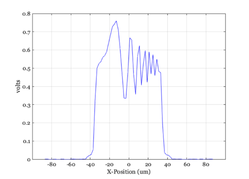
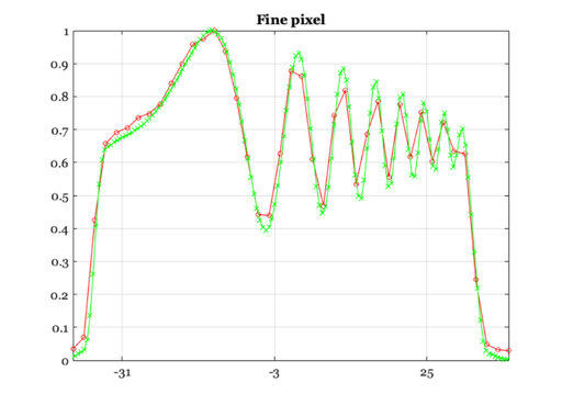
Illustration of pixel size (sensor spatial resolution) and aliasing
Deprecated. Will replace with s_sensorAliasing
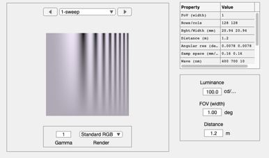
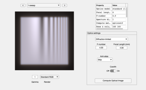
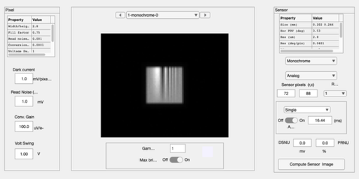
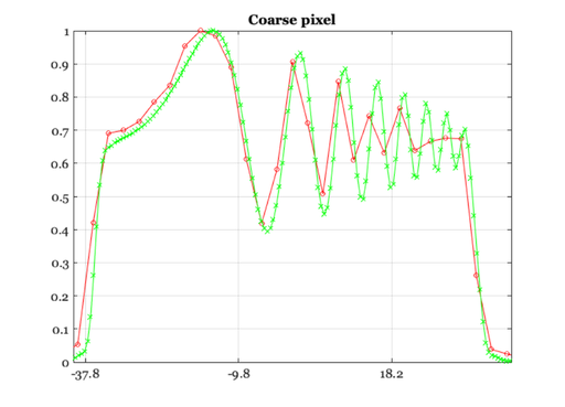
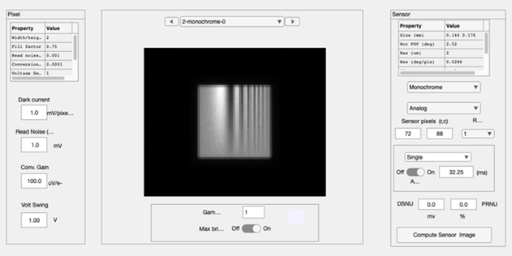
A sweep frequency scene is imaged through the optics to form an irradiance image. That image is then measured by a monochrome sensor with a coarse pixel and then with a fine pixel. The consequences of pixel size appear
See also: sensorCreate, sensorPlotLine
Copyright ImagEval Consultants, LLC, 2005.
Contents
- Create a scene with a simple test pattern and put it in the scene window
- Create an optical image and put it in the optical image window
- Create a monochrome sensor, and compute the voltage response
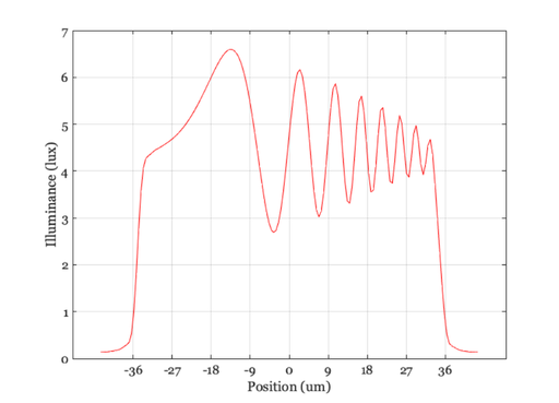
- Generate the optical image plot for illuminance
- Create a monochrome sensor with smaller pixels
- Same plotting as above, note the end of the aliasing
- END
ieInit
Create a scene with a simple test pattern and put it in the scene window
scene = sceneCreate('sweepFrequency');

% You can set the field of view in a variety of ways to alter the spatial
% scale of the optical image
scene = sceneSet(scene,'fov',1);
sceneWindow(scene);
Create an optical image and put it in the optical image window
oi = oiCreate;
oi = oiSet(oi,'optics fnumber',4);
oi = oiSet(oi,'optics focal Length',0.004);

oi = oiCompute(oi,scene);
oiWindow(oi);
Create a monochrome sensor, and compute the voltage response
sensor = sensorCreate('monochrome');
sensor = sensorCompute(sensor,oi);

% To see the sensor image in a GUI, use this
sensorWindow(sensor);

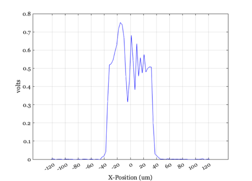
% Now plot the optical image and the voltage response on a common spatial
% scale. First, generate a plot of the voltage across the pixels on the
% sensor, saving the data in sData.  Choose the middle row.
row = sensorGet(sensor,'rows'); row = round(row/2);
[~, sData] = sensorPlotLine(sensor,'h','volts','space',[1,row]);
Generate the optical image plot for illuminance
row   = sceneGet(oi,'rows'); row = round(row/2);
oData = oiPlot(oi,'horizontal line illuminance',[1,row]);

% One set of data is in volts and the other in illuminance.  Normalize them
% to a common 0,1 range
sData.normData = ieScale(sData.pixData,0,1);
oData.normData = ieScale(oData.data,0,1);

% Now plot the two curves on the same spatial scale, remembering that the
% pixel position is in the middle.  That is why we take away 1/2 of the
% pixel width from the pixel position
% Plot the varying portion
ieNewGraphWin;
pSize = sensorGet(sensor,'pixel width','microns');
plot(sData.pixPos - pSize/2,sData.normData,'-o', ...
    oData.pos-1,oData.normData,'-x')
set(gca,'xlim',[-40 40])
xSpacing = 10*pSize;
xtick = min(sData.pixPos):xSpacing:max(sData.pixPos);
set(gca,'xtick',xtick); grid on; title('Coarse pixel')

% Notice the spatial aliasing at the high frequencies.
Create a monochrome sensor with smaller pixels
% Compute the voltage response ;
sensorSmall = sensorSet(sensor,'pixel size Constant Fill Factor',[1,1]*2e-6);
sensorSmall = sensorCompute(sensorSmall,oi);

% To see the sensor image in a GUI, use this
sensorWindow(sensorSmall);
Same plotting as above, note the end of the aliasing
row = sensorGet(sensorSmall,'rows'); row = round(row/2);

[~, sData] = sensorPlotLine(sensorSmall,'h','volts','space',[1,row]);

row = sceneGet(oi,'rows'); row = round(row/2);

[oData,g] = oiPlot(oi,'horizontallineilluminance',[1,row]);
if ~isdeployed % close gets an error when we run a Windows EXE
    close(g);
end
sData.normData = ieScale(sData.pixData,0,1);
oData.normData = ieScale(oData.data,0,1);
pSize = sensorGet(sensorSmall,'pixel width','microns');

ieNewGraphWin;
plot(sData.pixPos - pSize/2,sData.normData,'-o', ...
    oData.pos-1,oData.normData,'-x')
set(gca,'xlim',[-40 40])
xtick = min(sData.pixPos):xSpacing:max(sData.pixPos);
set(gca,'xtick',xtick); grid on; title('Fine pixel')
