Review of sensor estimation for spectral QE (Psych 221)

  Class:     Psych 221/EE 362
  Tutorial:  Sensor estimation procedure
  Author:    Wandell
  Purpose:   Introduce sensor responsivity, linear estimation,
    illuminant and surface functions, and sensor spectral estimation
  Date:      01.02.97
  Duration:  20 minutes

  Matlab 5:  Checked 01.06.98 BW
  Matlab 7:  Checked 01.04.08 BW

Copyright Imageval Consulting,

Contents

ieInit

Tutorial introduces several color calculations that are relevant to camera and scanner calibration. These calculations involve thinking about the sensors in the camer and scanner. As you perform the calculations, you should consider the relationship between how the scanner or camera encode light, and how the eye encodes light. Also, part of the tutorial will involve computations with surface reflectances and illuminants that are relevant to the Rendering tutorial.

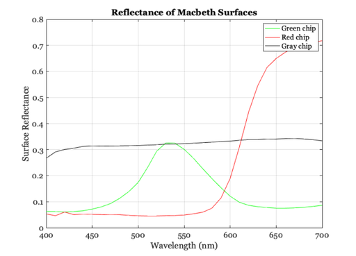
Surface Reflectance Functions

The Macbeth Color Checker is a set of 24 surfaces commonly used to evaluate color balancing systems. There is one in the ISEP lab. The surfaces that make up the Color Checker were selected to have the same surface reflectance functions as various important surfaces that are commonly used in television and film images. We will read in a matrix of data. Each row of the matrix is the reflectance function of one of the Macbeth surfaces, measured at each of 361 wavelength samples in the visible spectrum. (Most of the visible spectrum is in the 400-700 nanometers wavelength region.) Thus we get a 24x361 matrix of surface spectra. Each row is one surface.

% Load in the data representing the macbeth color checker surface
% reflectances.  The data are stored in the columns of the matrix.

wavelength = 400:10:700;
macbethChart = ieReadSpectra('macbethChart',wavelength);

% The different columns of this matrix represent various colored surfaces.
% The column numbers of some of the chips are

greenChip = 7; redChip = 11; whiteChip = 4; grayChip = 12;

% Let's look at the reflectance function of the green surface.

vcNewGraphWin;
plot(wavelength,macbethChart(:,greenChip),'g');grid on
xlabel('Wavelength (nm)');
ylabel('Surface Reflectance');
title('Reflectance of Macbeth Surfaces');

% Notice that about 18% of the light at wavelength 500 nm is
% reflected by the "Green" surface. Here is the reflectance
% function of a red surface:

hold on
plot(wavelength,macbethChart(:,redChip),'r');

% And here is a gray surface:

hold on
plot(wavelength,macbethChart(:,grayChip),'k');
legend('Green chip', 'Red chip','Gray chip')
hold off

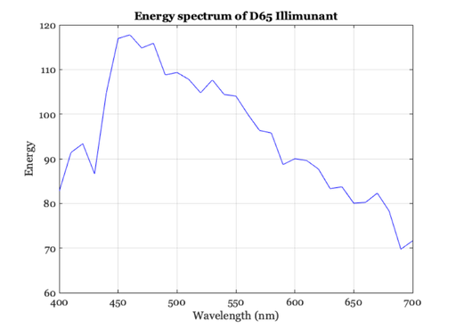
Creating a spectral power distribution of scattered light

This scattered light will be the signal encoded by the scanner.

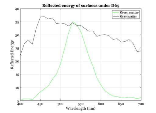
% Now, load in an illuminant.  The illuminant spd represent the
% amount of light present at each wavelength.

D65 = ieReadSpectra('D65.mat',wavelength);

% Make a plot of D65 a standard illuminant which represents a mix of blue
% sky and clouds.

vcNewGraphWin;
plot(wavelength,D65,'b'); grid on
xlabel('Wavelength (nm)');
ylabel('Energy');
title('Energy spectrum of D65 Illimunant');

% The light scattered from the surface is the pointwise product of the
% incident light and the reflectance of the surface at the each wavelength.
% There are lots of ways to do this calculation, but I find it simple to
% perform it for all of the surfaces at once as a matrix product.
%
% First, we turn the spd of the light into a diagonal matrix, and then we
% multiply that matrix times the matrix whose columns contain the surface
% reflectance functions.

spectral_signals = diag(D65)*macbethChart;

% As examples, plot the spectral signal scattered from the green and
% gray  Macbeth surfaces.

vcNewGraphWin;
plot(wavelength,spectral_signals(:,greenChip),'g'); hold on
plot(wavelength,spectral_signals(:,grayChip),'k');  hold off
xlabel('Wavelength (nm)'); ylabel('Reflected Energy');
title('Reflected energy of surfaces under D65')
legend('Green scatter','Gray scatter')
grid on

Predicting device sensor responses to the light sources

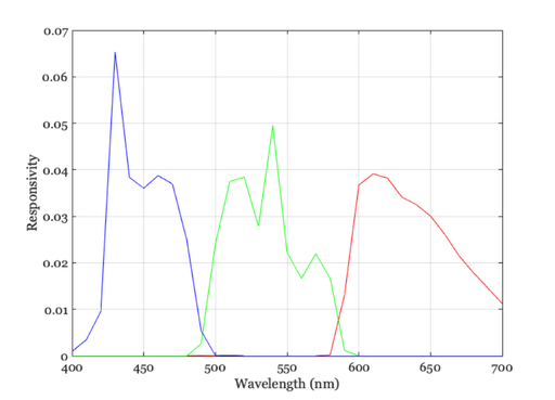
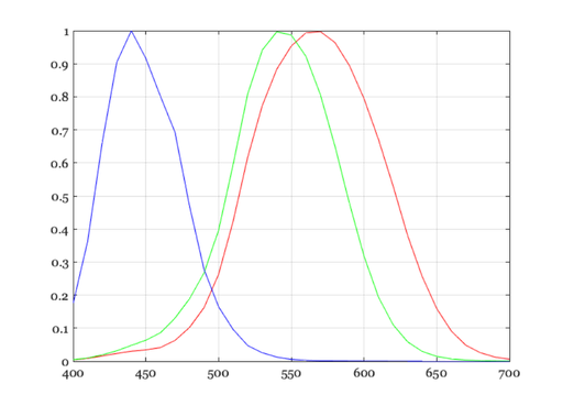
% Now, we calculate the expected response from a linear sensor given a
% particular spectral signal.  The spectral responsivitiy of the r,g,b
% sensors in an HP Scanjet IIC I once calibrated are contained in this
% file.

sensors = ieReadSpectra('cMatch/camera', wavelength);
plot(wavelength(:), sensors); grid on
xlabel('Wavelength (nm)'); ylabel('Responsivity')

% Take a look at the spectral responsivities of these sensors. Notice that
% they hardly overlap.  This non-overlapping structure is due to  the way
% the device is built, using dichroic filters, and I will explain this in
% class.  Most significantly, notice that these sensors really don't look
% anything like the cone sensitivities of the human eye.

ncones = ieReadSpectra('SmithPokornyCones',wavelength);
vcNewGraphWin;
plot(wavelength(:),ncones);
grid on

PREDICTING SENSOR RESPONSES TO D65 REFLECTED FROM MACBETH CHART

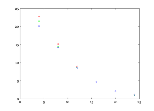
% We can predict the (linear) sensor responses by a simple matrix
% multiplication. The matrix product of the sensor sensitivites (in the
% rows) and the spectral signals (in the columns) generates the response
% for each sensor class.

rgbResponses= sensors'*spectral_signals;
size(rgbResponses)

% Notice the size of the rgb matrix.  It is 3 by 24 because there are three
% types of sensors and 24 surfaces in the Macbeth Color Checker.

% We can plot the rgb responses of this scanner to the light scattered from
% the gray surfaces.  Before we create this plot, ask yourself what you
% think the values ought to be.

% In order of lightest to darkest, here are the gray surfaces.
graySeries = 4:4:24;

% And here is how to plot the predicted rgb responses
%
plot(graySeries,rgbResponses(1,graySeries)','ro', ...
    graySeries,rgbResponses(2,graySeries)','go', ...
    graySeries,rgbResponses(3,graySeries)','bo')

ans =

     3    24

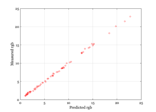
ESTIMATE THE SENSOR RESPONSIVITIES

% Suppose that we didn't know the spectral properties of the scanner.  How
% could we estimate the wavelength tuning of the sensors in the scanner by
% making a set of measurements? We might be able to measure the scanner
% illuminant directly, just by opening the box during the scan.  So,
% figuring out the illuminant should be pretty easy.

% Given the illuminant is known, how do we estimate the properties of the
% camera sensors?  We need to measure how the sensors respond to a
% calibrated target, like the Macbeth color-checker.  If we know the
% illuminant, then we can calculate the spectral signals arriving at the
% sensors.  We have calcuclated them already above as "spectral_signals."
% In general, we know that the rgbResponses are equal to

% rgbResponses = scanner'*spectral_signals

% Given that we know the spectral_signals and the rgbResponses and we want
% to estimate the scanner.  It might be helpful to draw a matrix tableau of
% what this equation represents.  You will see that there are more unknowns
% than there are linear equations. Hence, it is impossible to estimate the
% scanner sensitivity uniquely from these measurements.  But, we can
% measure that part of the scanner sensitivity that falls within the column
% space of the spectral signals.  We do this by calculating the
% "pseudo-inverse" of the matrix spectral_signals.

estimate = (rgbResponses*pinv(spectral_signals))';

plot(wavelength,estimate(:,1),'r', ...
    wavelength,estimate(:,2),'g', ...
    wavelength,estimate(:,3),'b')
grid on
xlabel('Wavelength'), ylabel('Responsivity')
title('Estimated sensor responses')

% Notice that even for this computational example, the estimates are not
% perfect: there are noticeable differences between them and the original
% sensors.  But, the estimated sensors predict the responses perfectly.

rgbPred = estimate'*spectral_signals;
plot(rgbPred(:),rgbResponses(:),'o')
grid on

% Suppose we had fewer measurements samples.  How well would we
% have done on the estimation?

l = 1:5:24;
estimate = (rgbResponses(:,l)*pinv(spectral_signals(:,l)))';

plot(wavelength,estimate(:,1),'r', ...
    wavelength,estimate(:,2),'g', ...
    wavelength,estimate(:,3),'b')
grid on
xlabel('Wavelength'), ylabel('Responsivity')
title('Estimated sensor responses')

% The new estimates are worse.  We might also ask how well the new
% estimates to in predicting the full set of responses, that is the
% responses to the surfaces not in the list, l.

rgbPred = estimate'*spectral_signals;
plot(rgbPred(:),rgbResponses(:),'o')
xlabel('Predicted rgb'); ylabel('Measured rgb');
grid on

% Try adding in some measurement noise to create a new estimate.
%
randn('seed',0);
n = 10*randn(size(rgbResponses));
sig = max(0,rgbResponses + n);
estimate = (sig(:,l)*pinv(spectral_signals(:,l)))';

Plot the estimate and the rgbPredictions to see how well we did.

Published with MATLAB® R2024a