Estimate color filter responsivities

Using a series of test spectral power distributions, we calculate the sensor response and estimate the color filter transmissivities.

Make a uniform scene

scene = sceneCreate('uniform ee');
wave  = sceneGet(scene,'wave');

oi = oiCreate('default',[],[],0);
oi = oiSet(oi,'optics model','diffraction limited');
oi = oiSet(oi,'optics fnumber',0.01);   % No blurring

sensor = sensorCreate;
sensor = sensorSet(sensor,'size',[64 64]);
sensor = sensorSet(sensor,'auto exposure',true);

% The scene must always be larger than the sensor field of view.
scene = sceneSet(scene,'fov',sensorGet(sensor,'fov',scene,oi)*1.5);

Generate SPDs to use in test scene

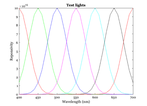
waveStep = 50;
cPos     = (wave(1):waveStep:wave(end));  % Center wavelengths
widths   = waveStep/2;
nLights  = length(cPos);

% These are Gaussian shaped SPDs.  cPos is the center position and widths
% is the width of the Gaussian.  You can plot them below.
spd = zeros(length(wave),nLights);
for ii=1:nLights
    spd(:,ii) = exp(-1/2*( (wave-cPos(ii))/(widths)).^2);
end
spd = spd*10^16;  % Make them a reasonable number

Show the SPDs

vcNewGraphWin;
plot(wave,spd);
xlabel('Wavelength (nm)');
ylabel('Reponsivity');
title('Test lights');

Create the series of spectral scenes and compute

% We compute the oi and the sensor, saving the data
eTime        = zeros(1,nLights);
nFilters     = sensorGet(sensor,'nfilters');
volts        = cell(1,nFilters);
responsivity = zeros(nFilters,nLights);

for ii=1:nLights

    % Make a scene with a particular spectral power distribution (spd). The
    % code has to arrange the data into the proper 3d matrix format.
    spdImage = repmat(spd(:,ii),[1,32,32]);
    spdImage = permute(spdImage,[2 3 1]);
    scene    = sceneSet(scene,'photons',spdImage);
    % ieAddObject(scene); sceneWindow;

    % Compute the optical image
    oi     = oiCompute(oi,scene);
    % ieAddObject(oi); oiWindow;

    % Compute the sensor response.
    sensor    = sensorCompute(sensor,oi,0);
    eTime(ii) = sensorGet(sensor,'Exposure Time','sec');
    % ieAddObject(sensor); sensorImageWindow;

    % Calculate volts/sec for each of the channels at this wavelength
    for jj=1:nFilters
        volts{jj} = sensorGet(sensor,'volts',jj);
        responsivity(jj,ii) = mean(volts{jj})/eTime(ii);  % volts/sec
    end
end

Estimate filters from the measurements

Use linear estimation to calculate filters from responsivities

  responsivity = filters*spd;

So figure that filters are weighted sums of the spd's

filters = wgt*spd'

Then, wgt = responsivity*inv(spd'*spd); filters = wgt*spd';

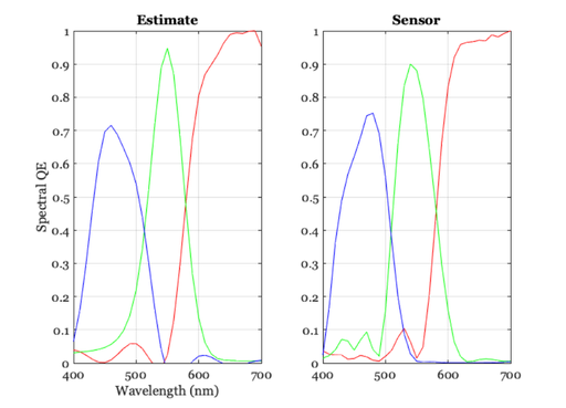
wgt = responsivity/(spd'*spd);  % Solve for weights
cFilters = (wgt*spd')';         % Solve for filters

% Normalize to peak of 1
cFilters = cFilters/max(cFilters(:));

% The estimates should match the sensor color filters
f = sensorGet(sensor,'color filters');
f = f/max(f(:));
vcNewGraphWin;
subplot(1,2,1), plot(wave,cFilters); grid on; set(gca,'ylim',[0 1])
title('Estimate'); xlabel('Wavelength (nm)'); ylabel('Spectral QE')
subplot(1,2,2), plot(wave,f); grid on; set(gca,'ylim',[0 1])
title('Sensor');

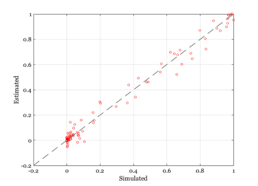
Compare directly

vcNewGraphWin;
plot(f(:),cFilters(:),'o');
identityLine;
xlabel('Simulated')
ylabel('Estimated');