Converts an image file into ISET sensor format

This script illustrate how to start with a raw image data from a camera, insert those data into the ISET pipeline, and then continue to explore using image quality evaluation and processing algorithms.

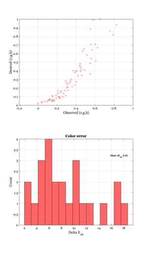
The script loads an MCC target offered up on the Internet. But the colors are not very good. We use sensorCCM to find the sensor color conversion matrix.

In this example, the color rendering of the original image is not very good, and in particular the distributed chart is saturated in the white regions. So the $\Delta E$ values are large.

ISET includes an accurate chart, which is how we can tell that the one from the Internet provided values that are not quite right. In the last section we see that those values have been 'gamma corrected', so they do not reflect the true sensor values. They need to be corrected by an exponent (2.2)

Read the TIF file
Create a matching sensor structure.
Attach the volts to the sensor
Interactively determine Color Conversion Matrix CCM
Render the image without the CCM
Render the image with the color conversion matrix
There is a nonlinearity

ieInit

Read the TIF file

% This is an approximation to the Gretag in some sensor.  It was
% distributed on the Internet.
fName = 'mccGBRGsensor.tif';
mosaic = imread(fName);   % We treat the data in this file as sensor volts
% imtool(mosaic)

Create a matching sensor structure.

% Simulated camera sensor is gbrg
sensor = sensorCreate('bayer (gbrg)');
sensor = sensorSet(sensor,'Name','Sensor demo');

Attach the volts to the sensor

We want to scale the digital values in the croppedMosaic so that the max is equal to the voltage swing and the min is equal to the dark level.

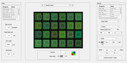
mn = double(min(mosaic(:)));
mx = double(max(mosaic(:)));
vSwing  = sensorGet(sensor,'pixel voltage swing');
volts = ((double(mosaic) - mn)/(mx - mn))*vSwing;
% figure; histogram(volts(:),50)

sensor = sensorSet(sensor,'size',size(volts));
sensor = sensorSet(sensor,'volts',volts);

%View the sensor voltages in the GUI
ieAddObject(sensor);
sensorWindow;

Interactively determine Color Conversion Matrix CCM

sensorCCM can be used interactively to find the rectangles. In that mode, you click on the outer corners of the patches in the order described in the message within the Sensor Window. When you are done, right click.

% But, you can just use this rectangle which lets this script run
% without user interaction.
cp = [
    15   584
    782   584
    784    26
    23    19];
sensor = sensorSet(sensor,'chart corner points',cp);
% [L,pointLoc] = sensorCCM(sensor,ccmMethod,pointLoc,showSelection)
sensorCCM(sensor,[],[],true);

% Notice the large $\Delta E$ values.  The sensor data from the
% Internet don't match our sensor.

Render the image without the CCM

% First, compute with the default properties.  This uses bilinear
% demosaicing, no color conversion or balancing.  The sensor RGB values are
% simply set to the display RGB values.

% Create a display image with basic attributes
ip = ipCreate;
ip = ipSet(ip,'name','No Correction');
ip = ipSet(ip,'scaledisplay',1);
ip = ipCompute(ip,sensor);
ieAddObject(ip);
ipWindow;

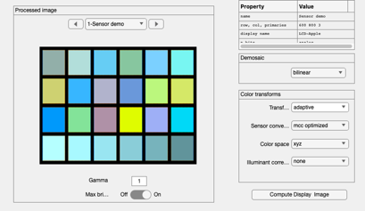
Render the image with the color conversion matrix

% For this data set, the white patch is saturated so the matrix isn't
% right.

ip = ipCreate;
ip = ipSet(ip,'name','CCM Correction');
ip = ipSet(ip,'scaledisplay',1);

% In the sensor window I used the pulldown under
%     Analyze | Color | Color Conversion Matrix
% to find an optimal linear transform for the sensor data to MCC
% values
m = [ ...
    0.9205   -0.1402   -0.1289
    -0.0148    0.8763   -0.0132
    -0.2516   -0.1567    0.6987];
ip = ipSet(ip,'conversion transform sensor',m);

% We set  the other transforms to the identity, so that the
% complete transform is just the one above.
ip = ipSet(ip,'correction transform illuminant',eye(3,3));
ip = ipSet(ip,'ics2Display Transform',eye(3,3));

% We set the ip to not ask any questions, just use the current matrices.
ip = ipSet(ip,'conversion method sensor ','current matrix');

% Compute and show.
ip = ipCompute(ip,sensor);
ieAddObject(ip); ipWindow;

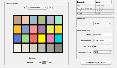
There is a nonlinearity

So this looks about right!

ip = ipSet(ip,'render gamma',2.2);
ieAddObject(ip); ipWindow;