Use linear models to approximate surface reflectances

Frequently we want to compress the spectral data. Linear models are one way to achieve good approximations to the original reflectance data but use many fewer numbers.

We create linear basis functions for the Gretag/Macbeth color checker surface reflectance functions. This script illustrates how to

Read reflectances
Create the basis functions
Approximate the original functions
Render images of the approximation

See also: ieReadSpectra, macbethReadReflectance, imageFlip

Read the Gretag/Macbeth ColorChecker reflectance spectra
Use SVD to create a linear model decomposition from the spectra
Illustrate the linear model approximations
Load XYZ and choose a light for the rendering experiments
Render the images from the lower dimensional models
Create the full rendering (no linear model approximation)

ieInit

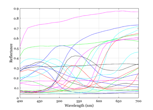
Read the Gretag/Macbeth ColorChecker reflectance spectra

% Read
wave = 400:10:700;    % nanometers
macbethReflectance = macbethReadReflectance(wave);

% Plot
vcNewGraphWin;
p = plot(wave,macbethReflectance);
set(p,'linewidth',1);
t = xlabel('Wavelength (nm)'); set(t,'fontname','Georgia')
t = ylabel('Reflectance'); set(t,'fontname','Georgia')
grid on

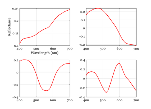
Use SVD to create a linear model decomposition from the spectra

% Build the linear model using the singular value decomposition
[U, S, V] = svd(macbethReflectance);

% It is also reasonable to build models by first removing the mean.
%  mn = mean(macbethReflectance,2);
%  tmp = macbethReflectance - repmat(mn,[1,size(macbethReflectance,2)]);
%  [U S V] = svd(tmp);
%  U = [mn(:), U(:,1:3)];
% These basis functions are a lot like the simple SVD functions.

% The columns of U are the basis functions It is nice to make them more
% positive than negative, on balance.
if sum(U(:,1)) < 0, U = -1*U; end

vcNewGraphWin;
for ii=1:4
    subplot(2,2,ii)
    p = plot(wave,U(:,ii)); set(p,'linewidth',2)
    grid on;
end
subplot(2,2,1)
t = xlabel('Wavelength (nm)'); set(t,'fontname','Georgia')
t = ylabel('Reflectance'); set(t,'fontname','Georgia')

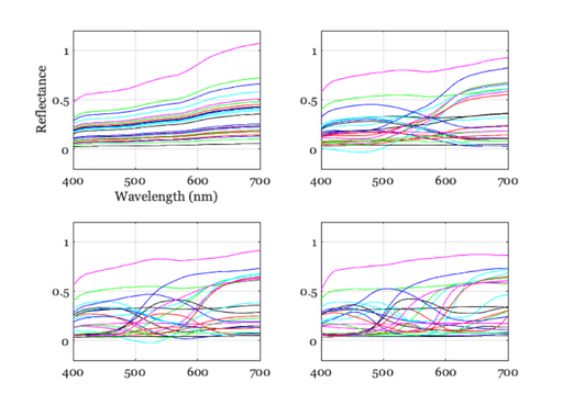
Illustrate the linear model approximations

[U, S, V] = svd(macbethReflectance);
W = S*V';
hdl = vcNewGraphWin;
for nDims=1:3
    subplot(2,2,nDims)
    list = 1:nDims;
    approxRef = U(:,list)*W(list,:);
    plot(wave,approxRef)
    set(gca,'fontName','Georgia')
    grid on
    set(gca,'ylim',[-0.2 1.2])
end

subplot(2,2,4)
plot(wave,macbethReflectance);
set(gca,'ylim',[-0.2 1.2])
grid on
set(gca,'fontName','Georgia')

subplot(2,2,1)
t = xlabel('Wavelength (nm)'); set(t,'fontname','Georgia')
t = ylabel('Reflectance'); set(t,'fontname','Georgia')

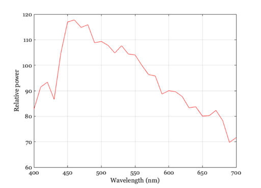
Load XYZ and choose a light for the rendering experiments

XYZ = ieReadSpectra('XYZ',wave);
lgt = ieReadSpectra('D65',wave);

% Plot the light
vcNewGraphWin;
plot(wave,lgt); grid on
xlabel('Wavelength (nm)'); ylabel('Relative power');

% Or try these lights instead
% lgt  = ieReadSpectra('tungsten',wave);
% lgt  = ieReadSpectra('FluorescentOffice',wave);
% lgt  = ieReadSpectra('Fluorescent2',wave);
% lgt  = ieReadSpectra('Fluorescent7',wave);
% lgt  = ieReadSpectra('Fluorescent11',wave);

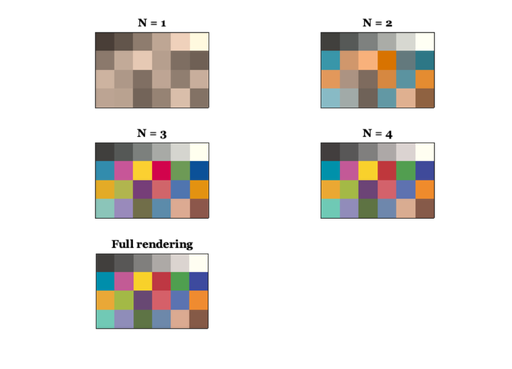
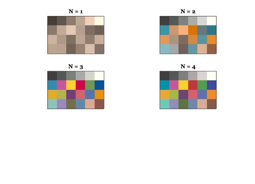
Render the images from the lower dimensional models

[U, S, V] = svd(macbethReflectance);
W = S*V';
vcNewGraphWin;
for nDims= 1:4  %5:8 %

    list = 1:nDims;

    % Render for this light, nDims, and set peak Y to 100
    mccXYZ = XYZ'*diag(lgt)*U(:,list)*W(list,:);
    mx = max(mccXYZ(2,:)); mccXYZ = 100*(mccXYZ/mx);

    % Pack it into an RGB format
    imRGB = xyz2srgb(XW2RGBFormat(mccXYZ',4,6));
    imRGB = imageFlip(imRGB,'updown');
    imRGB = imageFlip(imRGB,'leftright');

    %
    subplot(3,2,nDims)
    imagesc(imRGB); axis image
    set(gca,'xtick',[],'ytick',[])
    title(sprintf('N = %.0f',nDims))
end

Create the full rendering (no linear model approximation)

subplot(3,2,5)
mccXYZ = XYZ'*diag(lgt)*U*W;
mx = max(mccXYZ(2,:)); mccXYZ = 100*(mccXYZ/mx);
imRGB = xyz2srgb(XW2RGBFormat(mccXYZ',4,6));
imRGB = imageFlip(imRGB,'updown');
imRGB = imageFlip(imRGB,'leftright');
imagesc(imRGB); axis image
set(gca,'xtick',[],'ytick',[])
title(sprintf('Full rendering'))