Illuminant correction

Illuminant correction is often performed by calculating a 3x3 matrix that maps the XYZ values for surfaces under one light into the XYZ values under another light.

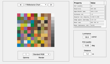
Here, we create a scene that consists of patches illuminated by light A these patches can be created by randomly sampling surfaces reflectances the selection of surfaces will matter

We then create another scene that consists of the same patches illuminated by light B

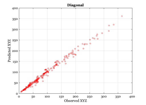
We calculate a general 3x3 matrix that maps the XYZ values for surfaces under light A into the XYZ values of surfaces under light B. We then find a 3x3 diagonal matrix that maps the XYZ values for surfaces under light A into the XYZ values of surfaces under light B.

The general 3x3 matrix does a better job than the diagonal (as expected).

Some authors refer to the diagonal 3x3 as von Kries adaptation Note that a matrix that is diagonal in one coordinate frame (XYZ) will not generally be diagonal in another coordinate frame (e.g., LMS or RGB). Von Kries meant diagonal in LMS.

See also: RGB2XWFormat

Copyright ImagEval Consultants, LLC, 2012.

Contents

ieInit

Create a test scene (Natural 100)

% Set the illumination to D65
scene = sceneCreate('reflectance chart');
sceneD65 = sceneAdjustIlluminant(scene,'D65.mat');
sceneD65 = sceneSet(sceneD65,'name','Reflectance Chart D65');
ieAddObject(sceneD65); sceneWindow;

Solve for matrix relating the chart under two different lights

% This are the surfaces under a D65 light
xyz1 = sceneGet(sceneD65,'xyz');

% This is a nSample x 3 representation of the surfaces under D65
xyz1 = RGB2XWFormat(xyz1);

This are the surfaces under a Tungsten light

sceneT = sceneAdjustIlluminant(scene,'Tungsten.mat');
xyz2   = sceneGet(sceneT,'xyz');

% This is a nSample x 3 representation of the surfaces under Tungsten
xyz2 = RGB2XWFormat(xyz2);

% We are looking for a 3x3 matrix, L, that maps
%
%    xyz1 = xyz2 * L
%    L = inv(xyz2'*xyz2)*xyz2'*xyz1 = pinv(xyz2)*xyz1
%
% Or, we just use the \ operator from Matlab for which inv(A)*B is A\B
L = xyz2 \ xyz1;

% To solve with just a diagonal, do it one column at a time
D = zeros(3,3);
for ii=1:3
    D(ii,ii) = xyz2(:,ii) \ xyz1(:,ii);
end

Plot predicted versus actual

vcNewGraphWin; pred2 = xyz2*L; plot(xyz1(:),pred2(:),'o'); grid on
title('Full inear'); xlabel('Observed XYZ'); ylabel('Predicted XYZ')

vcNewGraphWin; pred2 = xyz2*D; plot(xyz1(:),pred2(:),'o'); grid on
title('Diagonal'); xlabel('Observed XYZ'); ylabel('Predicted XYZ')

Published with MATLAB® R2024a