Illustrate how to create and interact with scenes

Simulations typically begin with a scene object. This script illustrates how to create a scene of the Macbeth ColorChecker illuminated with a D65 light. It then illustrates different ways to programmatically interact with the scene object.

We illustrate * how to display a downsampled (3 color channels) representation of the scene in the Display window. * Read properties of the scene using sceneGet . * Create a frequency-orientation scene target * Extract and plot scene luminance (cd/m^2) across a row of that target.

See also: sceneCreate, s_sceneFromMultispectral, s_sceneFromRGB

sceneCreate
sceneWindow
sceneGet
Plot the mean radiance
sceneDescriptions
Different types of scenes
END

ieInit;

% We validate some of the ISET calculations by the numerical tolerance
tolerance = 1e-5;

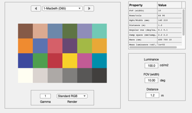
sceneCreate

% To create a simple spectral scene of a Macbeth Chart  under a
% D65 illuminant, we use
%
sceneMacbethD65 = sceneCreate('macbethd65');

sceneWindow

% To place the scene data in the window, add the scene object to
% the session and select it.
%
ieAddObject(sceneMacbethD65);
%
% Then bring up the scene window.  You can interact with the
% scene through this window
sceneWindow; pause(0.2);
%

sceneGet

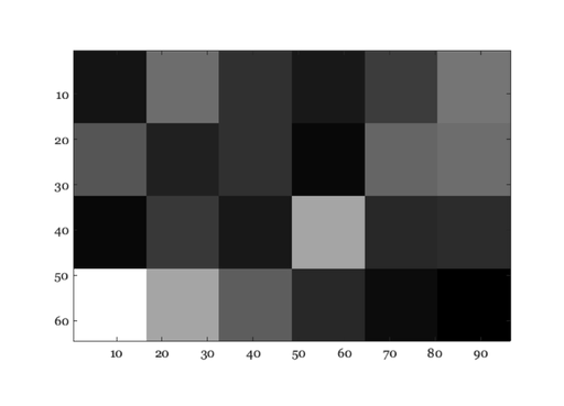
% To manipulate the data in a scene, you can extract variables
sceneGet(sceneMacbethD65,'meanLuminance')

% Image of the luminance map of the Macbeth
luminance = sceneGet(sceneMacbethD65,'luminance');

ieNewGraphWin;
imagesc(luminance); axis image; colormap(gray(64));

% To access directly the photons in the image, do this:
photons = sceneGet(sceneMacbethD65,'photons');

% This is a small image, but notice that it is row by col by
% wavelength
size(photons)

% The values are big because they are photons emitted per second
% per wavelength per steradian per meter from the scene
assert( abs(max(photons(:))/ 1.3119e+16 - 1) < tolerance,'Max photon error');

% These are the wavelength sample values in nanometers
wave = sceneGet(sceneMacbethD65,'wave');

% Suppose we compute the mean number of photons across the entire
% image
meanPhotons = mean(photons,1);  meanPhotons = mean(meanPhotons,2);
meanPhotons = squeeze(meanPhotons);
assert(abs(mean(meanPhotons(:)) / 3.7624e+15 - 1) < tolerance,'Mean photon error');

ans =

  100.0000


ans =

    64    96    31

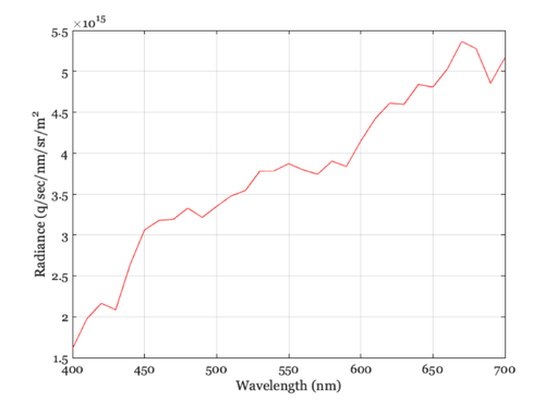
Plot the mean radiance

ieNewGraphWin;
plot(wave,meanPhotons);
xlabel('Wavelength (nm)'); ylabel('Radiance (q/sec/nm/sr/m^2');
grid on

sceneDescriptions

% To see a general description of the scene, the one printed in
% the upper right of the window, we use this
txt = sceneDescription(sceneMacbethD65);
disp(txt);

% Many other quantites can be stored or derived, such as the
% horizontal field of view in degrees
fprintf('FOV: %f\n',sceneGet(sceneMacbethD65,'fov'))

% To change the field of view
sceneMacbethD65 = sceneSet(sceneMacbethD65,'fov',20);
fprintf('FOV: %f\n',sceneGet(sceneMacbethD65,'fov'))

Row,Col:	64 by 96 
Hgt,Wdth	(139.98, 209.97) mm
Sample:	2.19 mm 
Deg/samp: 0.10
Wave:	400:10:700 nm
DR: 26.04 dB (max 320 cd/m2)

FOV: 10.000000
FOV: 20.000000

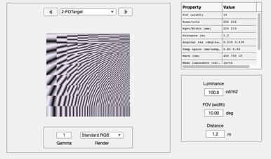
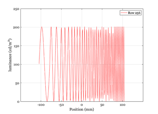
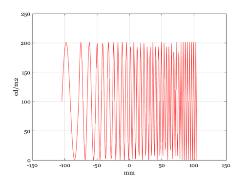
Different types of scenes

% There are many types of scenes.  Here is a simple one that is
% useful for demosaicing.  For a list, type help sceneCreate
sceneTest = sceneCreate('freq orient pattern');
sceneWindow(sceneTest); pause(0.2);

% With this one, we might try some simple plots, such as a plot
% of the luminance across the bottom row
sz = sceneGet(sceneTest,'size');
scenePlot(sceneTest,'luminance hline',sz);

% We can do this ourselves by getting the luminance of this
% bottom row as follows
luminance = sceneGet(sceneTest,'luminance');
data = luminance(sz(1),:);

support = sceneSpatialSupport(sceneTest,'mm');
ieNewGraphWin;
plot(support.x,data,'-');
xlabel('mm'); ylabel('cd/m2'); grid on

rows = round(sceneGet(sceneTest,'rows')/2);
assert(rows == 128,'Row test failed')
scenePlot(sceneTest,'radiance hline',[1,rows]);