Using the wvfPlot function

The wavefront toolbox uses Zernike polynomials to manage the optics. This script illustrates ways to create plots of the wvf data using the wvfPlot function.

Copyright Wavefront Toolbox Team, 2014-15

Contents

Initialize

ieInit;

Set up wfv object

wvf = wvfCreate;
wave = 550; wvf = wvfSet(wvf,'wave',wave);

% There is a bit of an art to setting the number of samples,
% because of reciprocal relation between sampling in pupil and
% retinal domains.  This choice is an OK compromise, but you can
% get finer results with additional fussing
wvf = wvfSet(wvf,'spatial samples',401);

% Compute the PSF
wvf = wvfCompute(wvf);

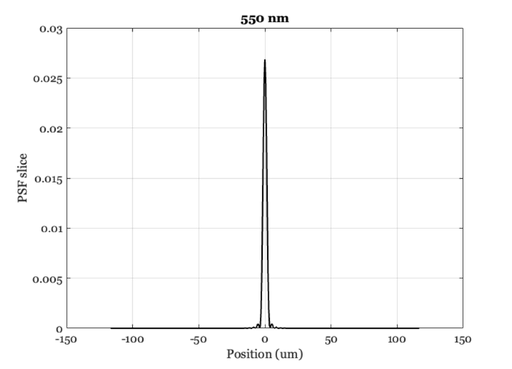
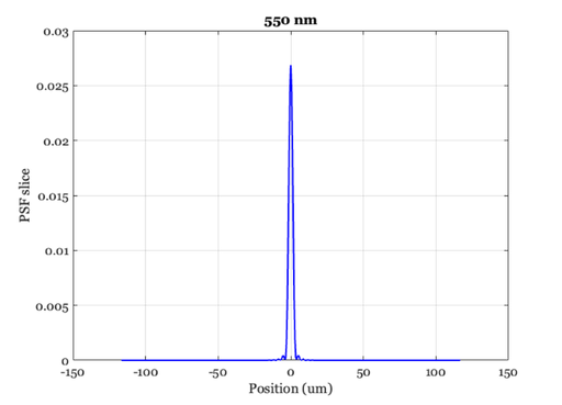
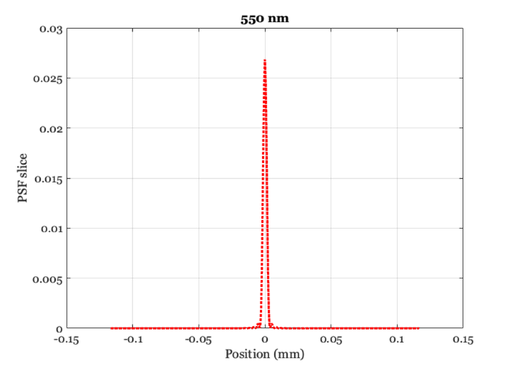
Make the plot in microns

unit = 'um';
[u,p]= wvfPlot(wvf,'1d psf','unit',unit,'wave',wave);
set(p,'color','k','linewidth',2)
title([num2str(wave) ' nm']);

% Normalize the plot
unit = 'um';
[u,p]= wvfPlot(wvf,'1d psf','unit',unit,'wave',wave);
set(p,'color','b','linewidth',2)
title([num2str(wave) ' nm']);

% Make the plot distance axis millimeters
unit = 'mm';
[u,p]= wvfPlot(wvf,'1d psf','unit',unit,'wave',wave);

set(p,'color','r','linewidth',3,'linestyle',':')
title([num2str(wave) ' nm']);

Show the return arguments

Data values that were plotted.

disp(u)

% Figure properties that can be set.
get(p)

    x: [-0.1166 -0.1160 -0.1155 -0.1149 -0.1143 -0.1137 … ] (1×401 double)
    y: [1.1658e-07 1.1560e-07 1.1281e-07 1.0670e-07 … ] (1×401 double)

      AffectAutoLimits: on
    AlignVertexCenters: off
            Annotation: [1×1 matlab.graphics.eventdata.Annotation]
          BeingDeleted: off
            BusyAction: 'queue'
         ButtonDownFcn: ''
              Children: [0×0 GraphicsPlaceholder]
              Clipping: on
                 Color: [1 0 0]
             ColorMode: 'manual'
           ContextMenu: [0×0 GraphicsPlaceholder]
             CreateFcn: ''
       DataTipTemplate: [1×1 matlab.graphics.datatip.DataTipTemplate]
             DeleteFcn: ''
           DisplayName: ''
      HandleVisibility: 'on'
               HitTest: on
         Interruptible: on
              LineJoin: 'round'
             LineStyle: ':'
         LineStyleMode: 'manual'
             LineWidth: 3
                Marker: 'none'
       MarkerEdgeColor: 'auto'
       MarkerFaceColor: 'none'
         MarkerIndices: [1 2 3 4 5 6 7 8 9 10 11 12 13 14 15 … ] (1×401 uint64)
            MarkerMode: 'auto'
            MarkerSize: 6
                Parent: [1×1 Axes]
         PickableParts: 'visible'
              Selected: off
    SelectionHighlight: on
           SeriesIndex: 1
           SourceTable: [0×0 table]
                   Tag: ''
                  Type: 'line'
              UserData: []
               Visible: on
                 XData: [-0.1166 -0.1160 -0.1155 -0.1149 … ] (1×401 double)
             XDataMode: 'manual'
           XDataSource: ''
             XVariable: ''
                 YData: [1.1658e-07 1.1560e-07 1.1281e-07 … ] (1×401 double)
             YDataMode: 'manual'
           YDataSource: ''
             YVariable: ''
                 ZData: [1×0 double]
             ZDataMode: 'auto'
           ZDataSource: ''
             ZVariable: ''

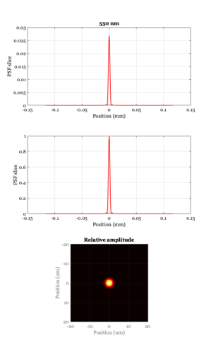
A multiple axis window

ieNewGraphWin([],'tall');
subplot(3,1,1), wvfPlot(wvf,'1d psf','unit',unit,'wave',wave,'window',false);
title([num2str(wave) ' nm']);
subplot(3,1,2), wvfPlot(wvf,'1d psf normalized','unit',unit,'wave',wave,'window',false);
subplot(3,1,3), wvfPlot(wvf,'image psf','unit','um','wave',wave,'plot range', 20, 'window',false);

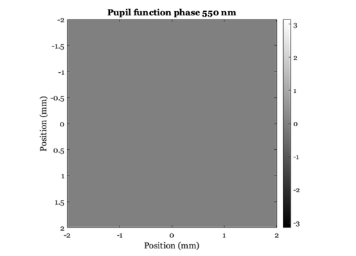
Pupil amplitude and phase

unit = 'mm'; maxMM = 2;
wvfPlot(wvf,'image pupil amp','unit',unit,'wave',wave,'plot range',maxMM);
title(['Pupil function amplitude ' num2str(wave) ' nm']);
wvfPlot(wvf,'image pupil phase','unit',unit,'wave',wave,'plot range',maxMM);
title(['Pupil function phase ' num2str(wave) ' nm']);

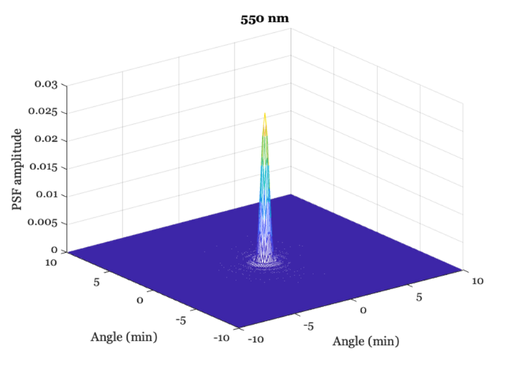
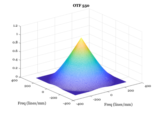
Mesh plots of the psf in angle and space

unit = 'min'; maxMIN = 10;
wvfPlot(wvf,'2d psf angle','unit',unit,'wave',wave,'plot range',maxMIN);

title([num2str(wave) ' nm']);

unit = 'mm'; maxMM = .050;
wvfPlot(wvf,'psf','unit',unit,'wave',wave,'plot range',maxMM);

title([num2str(wave) ' nm']);

% These are linepairs / unit and maximum frequency
unit = 'mm'; maxF = 300;
wvfPlot(wvf,'2d otf','unit',unit,'wave',wave,'plot range',maxF);

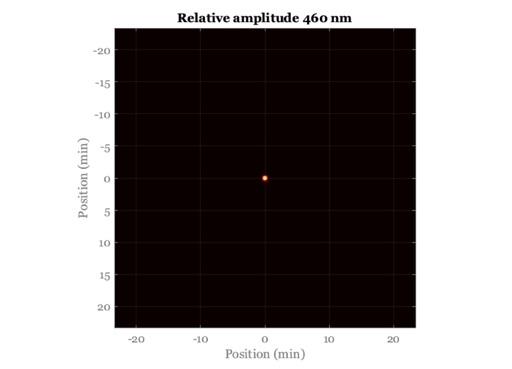
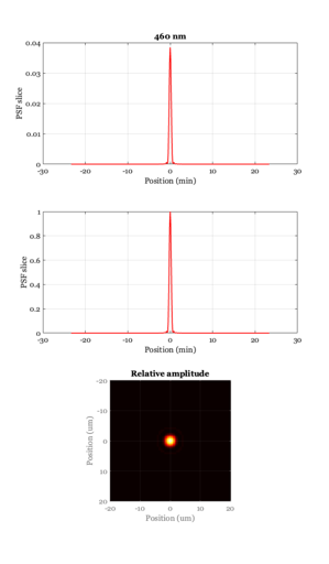
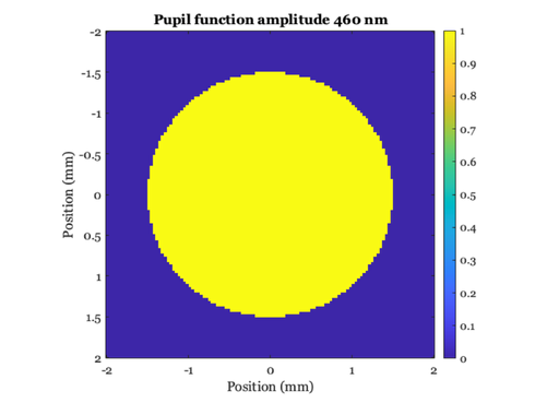
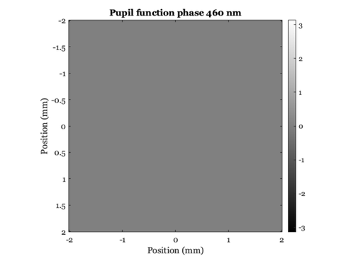
Change the calculated PSF wavelength and plot again

% Notice that we don't get an Airy disk, because the calculation
% includes chromatic aberrations.  These show up in the optical
% phase plot in the pupil plane.
%
% Another way to say this is that the pupil function is specified
% at a measurement wavelength, and when we calculate at different
% wavelengths a model of defocus is applied according to a model
% of the human eye's chromatic aberrations.

wave = 460; wvf = wvfSet(wvf,'wave',wave);
wvf = wvfCompute(wvf);
unit = 'min';
wvfPlot(wvf,'image psf angle','unit',unit,'wave',wave);

title(['Relative amplitude ' num2str(wave) ' nm']);

% A multiple axis window
ieNewGraphWin([],'tall');
subplot(3,1,1), wvfPlot(wvf,'1d psf','unit',unit,'wave',wave,'window',false);
title([num2str(wave) ' nm']);
subplot(3,1,2),
wvfPlot(wvf,'1d psf normalized','unit',unit,'wave',wave,'window',false);
subplot(3,1,3), wvfPlot(wvf,'image psf','unit','um','wave',wave,'plot range',20,'window',false);

% Pupil amplitude and phase
unit = 'mm'; maxMM = 2;
wvfPlot(wvf,'image pupil amp','unit',unit,'wave',wave,'plot range',maxMM);
title(['Pupil function amplitude ' num2str(wave) ' nm']);
wvfPlot(wvf,'image pupil phase','unit',unit,'wave',wave,'plot range',maxMM);
title(['Pupil function phase ' num2str(wave) ' nm']);

Published with MATLAB® R2024a