Create a shift-invariant, ideal, optics

Many optics calculations in ISET use some type of shift-invariant calculation. For example, diffraction limiated is a special case of ideal shift-invariant optics that achieves the best physically realizable image for a real lens.

The general shift-invariant case can specify any optical transfer function (OTF) or PSF. The default shift-invariant system is a simple pillbox SI. But we can create other examples, as well.

This script illustrates several shift-invariant systems, including one that is better than any physically realizable system. To show this case, we assign an OTF that passes all spatial frequencies, without any loss. Then we create a diffraction-limited OTF.

We also create a much blurrier OTF with a Gaussian shape.

Copyright Imageval Consulting, LLC 2016

Contents

ieInit

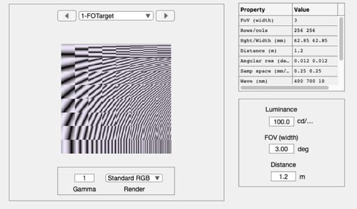
First a test scene

scene = sceneCreate('frequency orientation');
scene = sceneSet(scene,'fov',3);
ieAddObject(scene);
sceneWindow;

Now, create a simple shift-invariant OI with default parameters

% The default is a pillbox.  Perhaps it should be a Gaussian.
oi = oiCreate('shift invariant');
oi = oiCompute(oi,scene);
oi = oiSet(oi,'name','SI pillbox');

ieAddObject(oi); oiWindow;
fNumber = oiGet(oi,'optics fnumber');
oiPlot(oi,'PSF 550');

Now, replace the OTF with all ones, which is better than diffraction

% Get the original OTF of diffraction case and save for later use
OTF = oiGet(oi,'optics OTF');
nSamples = size(OTF,1);
nWave    = size(OTF,3);

% Replace OTF with all ones
iOTF = ones(size(OTF));
oiIdeal = oiSet(oi,'optics OTF',iOTF);

% Compute away
oiIdeal = oiCompute(oiIdeal,scene);
oiIdeal = oiSet(oiIdeal,'name','Ideal');
ieAddObject(oiIdeal); oiWindow;

% Show the point spread function
oiPlot(oiIdeal,'PSF 550');

Create the diffraction-limited case with the same fnumber

oiD = oiCreate('diffraction limited');
oiD = oiSet(oiD,'optics fnumber',fNumber);
oiD = oiCompute(oiD,scene);
oiD = oiSet(oiD,'name','Diffraction');

ieAddObject(oiD); oiWindow;
oiPlot(oiD,'PSF 550');

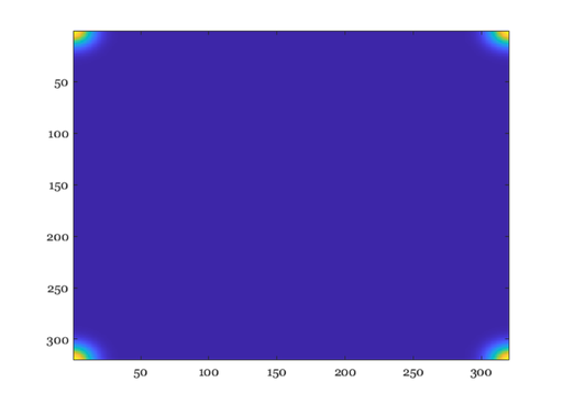
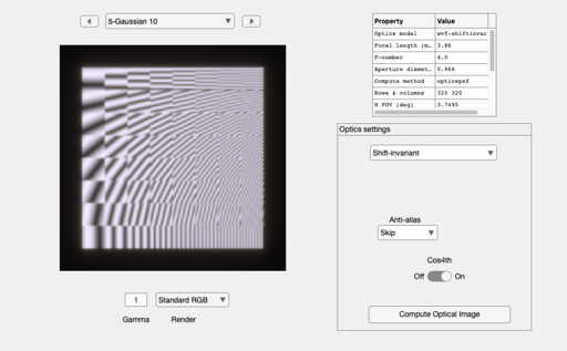
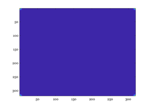
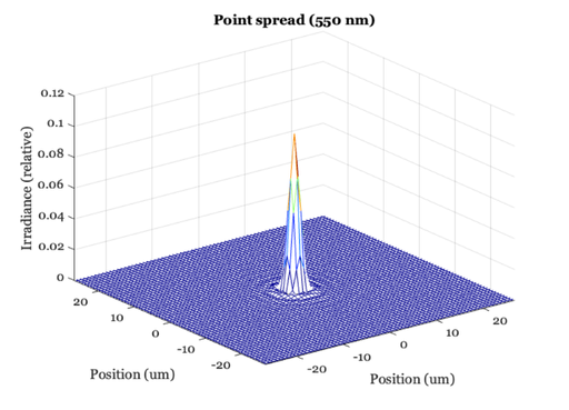
Gaussian example, no chromatic aberration

% Increasing the Gaussian sigma of the OTF sharpens the image
for sigma = [3 10]

    % A Gaussian
    g = fspecial('gaussian',[nSamples nSamples],sigma);

    % The (1,1) position is in the upper left corner
    g = fftshift(g);
    vcNewGraphWin; imagesc(g)

    % Replicate and set
    gOTF = repmat(g, [1 1 nWave]);
    oiG = oiSet(oi,'optics OTF',gOTF);
    oiG = oiSet(oiG,'optics fnumber',fNumber);

    % Compute
    oiG = oiCompute(oiG,scene);
    oiG = oiSet(oiG,'name',sprintf('Gaussian %.0f',sigma));
    ieAddObject(oiG); oiWindow;

    % Show the PSF, too
    oiPlot(oiG,'PSF 550');
end

Published with MATLAB® R2024a