Shift-invariant optics examples

This script illustrates how to create shift-invariant optics. The diffraction-limited optics is a special case in which the point spread function is derived. This is the more general case where the shape of the point spread function can be anything.

This code shows how to create the point spread functions for each wavelength place them in an optics structure and then optical image data structure. We then calculate the effect of the optics on a simple image and display the result in an optical image window.

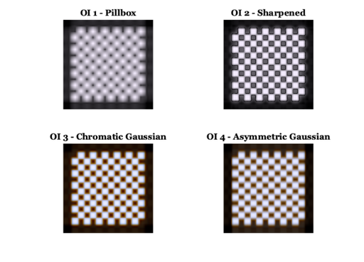
There are four example PSF. One is a simple pillbox (averaging) PSF. The second is a simple sharpening filter (difference of Gaussians). The third is a series of Gaussian blur filters with a spread that changes with wavelength. The fourth is an asymmetric Gaussian, with a wider x- than y-dimension.

Create the scene
Example 1: Create a pillbox point spread function
Read the psf and copy it into the optics slot of the oi
Example 2: A sharpening filter
Example 3: A Gaussian PSF that changes with wavelength
An asymmetric shift invariant psf
This may not be doing the right thing
Compare multiple oi images
End

ieInit

Create the scene

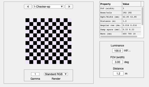
First, we create a checkerboard scene to blur.

pixPerCheck = 16;
nChecks = 6;
scene = sceneCreate('checkerboard',pixPerCheck,nChecks);
wave  = sceneGet(scene,'wave');
scene = sceneSet(scene,'fov',3);

% Replace the optical image into your ISET window
sceneWindow(scene);

Example 1: Create a pillbox point spread function

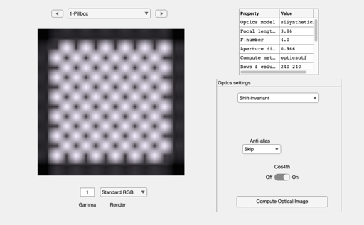
Point spread functions are small images. There is one image for each wavelength. In this example, the spatial grid is 128 x 128 with samples spaced every 0.25 microns. Hence, the image size is 128 * 0.25 = 32 microns on a side.

We create a point spread for each wavelength, 400:10:700. We write out a file that contains the point spread functions using ieSaveSIDataFile.

umPerSample = [0.5,0.5];                % Sample spacing

% Point spread is a little square in the middle of the image
h = zeros(128,128); h(48:79,48:79) = 1; h = h/sum(h(:));
psf = zeros(128,128,length(wave));
for ii=1:length(wave), psf(:,:,ii) = h; end     % PSF data

% Save the data
psfFile = fullfile(tempdir,'SI-pillbox');
ieSaveSIDataFile(psf,wave,umPerSample,psfFile);

Read the psf and copy it into the optics slot of the oi

After you compute, use the menu Analyze | Optics | <> in the oiWindow to plot various properties of the optics.

oi = oiCreate;
optics = siSynthetic('custom',oi,psfFile,[]);

% Attach the optics to the oi (optical image)
oi = oiSet(oi,'optics',optics);

% Setthe model to shift invariant
oi = oiSet(oi,'optics model','shiftInvariant');

% Apply the optics to the checkerboard scene.
oi = oiCompute(oi,scene);
oi = oiSet(oi,'name','Pillbox');

% Add to the database and show the OI window
ieAddObject(oi); oiWindow;

Example 2: A sharpening filter

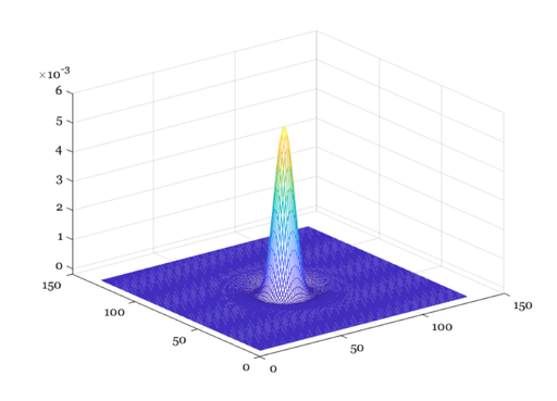
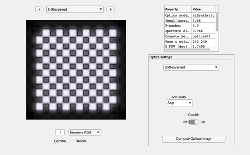
Now, we build a difference of Gaussians that will sharpen the original image a little. This is the psf.

h1 = fspecial('gaussian', 128, 5);
h2 = fspecial('gaussian', 128, 10);
h = h1 - 0.5*h2;
vcNewGraphWin; mesh(h)
psf = zeros(128,128,length(wave));
for ii=1:length(wave), psf(:,:,ii) = h; end     % PSF data

psfFile = fullfile(tempdir,'customFile');
% Save the data and all the rest, in compact form
ieSaveSIDataFile(psf,wave,umPerSample,psfFile);

optics = siSynthetic('custom',oi,psfFile,[]);
oi     = oiSet(oi,'optics',optics);
oi     = oiSet(oi,'optics model','shiftInvariant');

oi = oiCompute(oi,scene);
oi = oiSet(oi,'name','Sharpened');
oiWindow(oi);

Example 3: A Gaussian PSF that changes with wavelength

The spread of the Gaussian increases with wavelength, so the long wavelength PSF is much blurrier than the short wavelength PSF. Look for the color fringing in the oiWindow.

wave    = oiGet(oi,'wave');
psfType = 'gaussian';
waveSpread = (wave/wave(1)).^3;

% Make point spreads with a symmetric Gaussian
xyRatio = ones(1,length(wave));

% Now call the routine with these parameters
optics  = siSynthetic(psfType,oi,double(waveSpread),xyRatio);
oi      = oiSet(oi,'optics',optics);

% Here is the rest of the computation, as above
oi  = oiSet(oi,'optics model','shiftInvariant');
scene   = ieGetObject('scene');
oi      = oiCompute(oi,scene);

oi = oiSet(oi,'name','Chromatic Gaussian');
oiWindow(oi);

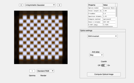
An asymmetric shift invariant psf

Notice that the checks appear a little wider than tall. In the oiWindow, use

Analyze | Optics | PSF Mesh to see the point spread a different wavelengths
Analyze | Line x Wave Plot to see the loss of contrast a long wavelengths compared to short wavelengths

This may not be doing the right thing

We need to make the wavelength dependence larger

fullName = fullfile(isetRootPath,'data','optics','si2x1GaussianWaveVarying.mat');
oi = ieGetObject('oi');
tmp = load(fullName);
oi = oiSet(oi,'optics',tmp.optics);
oi = oiSet(oi,'optics name','Gaussian Wave');
oi = oiCompute(oi,scene);
oi = oiSet(oi,'name','Asymmetric Gaussian');
oiWindow(oi);

Compare multiple oi images

This function lets you compare the image from all of the computed optical images.

imageMultiview('oi',1:4,1);