Color metrics tutorial (Psych 221)
  Class:     Psych 221/EE 362
  Tutorial:  Color metrics
  Author:    Wandell
  Purpose:   Introduce CIELAB metric and some of its uses.
  Date:      01.12.98
  Revised:   05.03.99 by Michael Bax
  Checked:   Matlab 7, GN, BW, 2006
  Modified for ISET, 2013 (BW).  More to do on this.
Duration: 30 minutes
This tutorial explores properties of the CIELAB color metric. In this tutorial, you will
- calculate CIELAB values for some simple surfaces and lights
- plot the relationship between linear intensity values and L*
- render CIELAB values on the screen
- calculate delta E values in a simple example
Contents
- Examine properties of the CIELAB color metric.
- Load a light source.
- Compute their XYZ values
- Here are the gray surfaces plotted in the 3-dimensional XYZ color space:
- Convert these values to LAB values.
- Plot in 3 dimensions for LAB space.
- Examine the chromaticity coordinates of these various surfaces.
- Creating and rendering the Lab values
- Some plots
- Render these XYZ values.
- Compute the linear rgb values for the collection of
- Have a look
- Show examples of LAB varying images
- Create the varyBstar values
- The Delta E_ab value
- End of tutorial
- BEGIN TUTORIAL QUESTIONS --
- END TUTORIAL QUESTIONS --
ieInit
Examine properties of the CIELAB color metric.
This metric is designed to help predict the discriminability between spatially uniform targets.
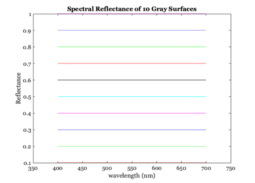
% Let's assume we have a set of gray surfaces whose reflectance
% functions are linearly scaled with respect to one another.
wavelength = 400:700;
graySurfaces = ones(length(wavelength),10)*diag([.1:.1:1]);

vcNewGraphWin;
plot(wavelength,graySurfaces)
set(gca,'xlim',[350 750]);
xlabel('wavelength (nm)'); ylabel('Reflectance')
title('Spectral Reflectance of 10 Gray Surfaces');
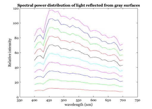
Load a light source.
D65 refers to the color temperature, namely 6500 deg Kelvin. This is a slightly bluish appearing light source.
lgt = ieReadSpectra('D65',wavelength);

% Illuminate the surfaces with the light source and plot the
% resulting scattered light
%
graySPD = diag(lgt)*graySurfaces;

vcNewGraphWin;
plot(wavelength,graySPD)
set(gca,'xlim',[350 750]);
xlabel('wavelength (nm)'); ylabel('Relative intensity')
title('Spectral power distribution of light reflected from gray surfaces');
Compute their XYZ values
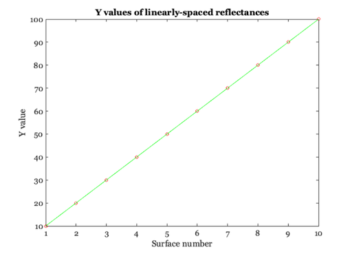
XYZ = ieReadSpectra('XYZ',wavelength);
grayXYZ = XYZ'*graySPD

% Remember:  the Y value of a white surface is always 100, so we
% must scale the results by the Y value of the white surface,
% appropriately.  The second row is Y, and the tenth surface is white.

grayXYZ = grayXYZ * 100 / grayXYZ(2,10)

% To compute the CIELAB values, we will need to use the XYZ values
% of the white surface.  So, let's save them in a special
% variable.

whiteXYZ = grayXYZ(:,10)

% Notice that the Y values of these 10 surfaces are linearly
% spaced.  That is because Y is a linear computation from the
% SPD.  The X and Z values are linear, too (not shown).
grayXYZ =

   1.0e+04 *

  Columns 1 through 7

    0.1003    0.2005    0.3008    0.4010    0.5013    0.6015    0.7018
    0.1056    0.2113    0.3169    0.4225    0.5281    0.6338    0.7394
    0.1147    0.2293    0.3440    0.4587    0.5734    0.6880    0.8027

  Columns 8 through 10

    0.8020    0.9023    1.0025
    0.8450    0.9506    1.0563
    0.9174    1.0320    1.1467


grayXYZ =

  Columns 1 through 7

    9.4912   18.9824   28.4736   37.9648   47.4561   56.9473   66.4385
   10.0000   20.0000   30.0000   40.0000   50.0000   60.0000   70.0000
   10.8563   21.7125   32.5688   43.4250   54.2813   65.1375   75.9938

  Columns 8 through 10

   75.9297   85.4209   94.9121
   80.0000   90.0000  100.0000
   86.8500   97.7063  108.5625


whiteXYZ =

   94.9121
  100.0000
  108.5625
vcNewGraphWin;
plot(1:10, grayXYZ(2,:),'o',1:10,grayXYZ(2,:),'-')
xlabel('Surface number'); ylabel('Y value')
title('Y values of linearly-spaced reflectances');
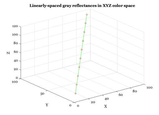
Here are the gray surfaces plotted in the 3-dimensional XYZ color space:
vcNewGraphWin;
plot3(grayXYZ(1,:), grayXYZ(2,:), grayXYZ(3,:),'o',...
    grayXYZ(1,:), grayXYZ(2,:), grayXYZ(3,:),'-');
xlabel('X'); ylabel('Y'); zlabel('Z');
title('Linearly-spaced gray reflectances in XYZ color space');
grid on;
Convert these values to LAB values.
We call the routine ieieXYZ2LAB. You should take a look at the routine to see what it does by invoking "type ieieXYZ2LAB"
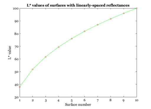
grayLAB = ieXYZ2LAB( grayXYZ.', whiteXYZ.' ).'

% Let's plot the L* values of these gray surfaces.  This set of values is
% not linearly related to the surface reflectance functions.  Rather, they
% are related by a cube root function.
vcNewGraphWin;
plot(1:10,grayLAB(1,:),'o',1:10,grayLAB(1,:),'-');
xlabel('Surface number');ylabel('L* value')
title('L* values of surfaces with linearly-spaced reflectances');
grayLAB =

  Columns 1 through 7

   37.8424   51.8372   61.6542   69.4695   76.0693   81.8382   86.9969
    0.0000    0.0000    0.0000         0         0    0.0000    0.0000
   -0.0000   -0.0000   -0.0000   -0.0000         0   -0.0000   -0.0000

  Columns 8 through 10

   91.6849   95.9968  100.0000
    0.0000         0         0
   -0.0000   -0.0000         0
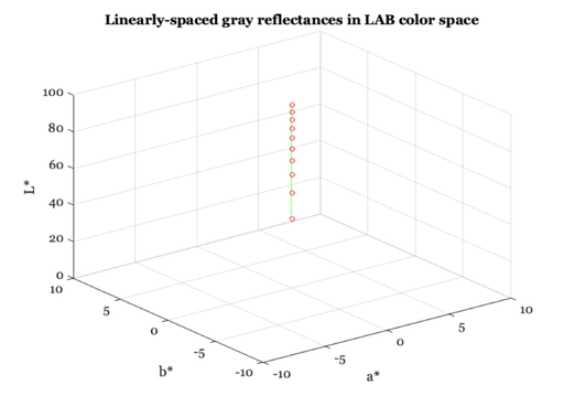
Plot in 3 dimensions for LAB space.
Notice that the a* and b* coordinates are zero for the gray series.
vcNewGraphWin;
plot3(grayLAB(2,:), grayLAB(3,:), grayLAB(1,:),'o',...
    grayLAB(2,:), grayLAB(3,:), grayLAB(1,:),'-');
xlabel('a*'); ylabel('b*'); zlabel('L*');
title('Linearly-spaced gray reflectances in LAB color space');
grid on; axis([ -10 10 -10 10 0 100]);
Examine the chromaticity coordinates of these various surfaces.
Remember that the chromaticity coordinates represent only two of the three dimensions. In this case, the surfaces all share a common "shape" spectral power distribution, and they differ only by a scale factor. So the surfaces will have the same chromaticity coordinates.
grayxy = chromaticity(grayXYZ')'
grayxy =

  Columns 1 through 7

    0.3128    0.3128    0.3128    0.3128    0.3128    0.3128    0.3128
    0.3295    0.3295    0.3295    0.3295    0.3295    0.3295    0.3295

  Columns 8 through 10

    0.3128    0.3128    0.3128
    0.3295    0.3295    0.3295
Creating and rendering the Lab values
% The a* and b* describe aspects of the hue and saturation of the
% targets For the gray series, the values of a* and b* (the 2nd
% and third rows of grayLAB) are all near zero.  Next, we use the
% methods we developed in the ColorMatching tutorial to create
% new Lab values and render them on the screen.
%

% Let's make a list of Lab values that are the same as the gray
% values, but that systematically vary the a* range.
%

nChips = size(grayLAB,2);
aRamp = ieScale(1:nChips,-30,30);
varyAstarLAB = zeros([3, nChips]);
varyAstarLAB(1,:) = 70;    % L
varyAstarLAB(2,:) = aRamp; % A = linear ramp
varyAstarLAB(3,:) = 0;
varyAstarLAB

% To see what these Lab values look like, we will (a) convert the Lab
% values into XYZ values, (b) guess about your screen primary spectral
% power distributions and gamma to render these XYZ values.  The techniques
% we use here are the same as in the ColorMatching.m tutorial.

% First, use this function to invert the LAB values to XYZ
% values.  Notice that we need to know the white point, whiteXYZ.

varyXYZ = ieLAB2XYZ(varyAstarLAB',whiteXYZ)'

% Stop for just a moment to see how varying the value of a*
% changes the chromaticity values.  Using the XYZ values, we can
% calculate the chromaticity values.  Notice that as we vary a*
% the chromaticity values move along a simple path.
varyxy = chromaticity(varyXYZ')';
varyAstarLAB =

  Columns 1 through 7

   70.0000   70.0000   70.0000   70.0000   70.0000   70.0000   70.0000
  -30.0000  -23.3333  -16.6667  -10.0000   -3.3333    3.3333   10.0000
         0         0         0         0         0         0         0

  Columns 8 through 10

   70.0000   70.0000   70.0000
   16.6667   23.3333   30.0000
         0         0         0


varyXYZ =

  Columns 1 through 7

   30.0254   31.8227   33.6904   35.6297   37.6421   39.7289   41.8914
   40.7494   40.7494   40.7494   40.7494   40.7494   40.7494   40.7494
   44.2386   44.2386   44.2386   44.2386   44.2386   44.2386   44.2386

  Columns 8 through 10

   44.1310   46.4490   48.8468
   40.7494   40.7494   40.7494
   44.2386   44.2386   44.2386
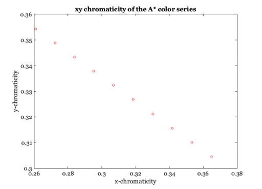
Some plots
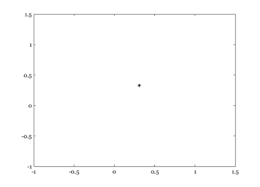
vcNewGraphWin;
plot(varyxy(1,:),varyxy(2,:),'o'); hold on
xlabel('x-chromaticity'),ylabel('y-chromaticity')
title('xy chromaticity of the A* color series');

% Let's see where the chromaticity point of white is.
whitexy = chromaticity(whiteXYZ')'
vcNewGraphWin;
plot(whitexy(1),whitexy(2),'k*'); hold off
whitexy =

    0.3128
    0.3295
Render these XYZ values.
We must load up some calibration information about your monitor. Because I have no idea what monitor you are using -- this is a general problem for the industry -- I am going to just make a guess and use a standard set of monitor values.
d = displayCreate('LCD-Apple','wave',wavelength);

% Now, compute the transformations from XYZ to linear rgb and
% back for this monitor
rgb2xyz = displayGet(d,'rgb2xyz');  % Display primary spectral power distribution
xyz2rgb = inv(rgb2xyz);
Compute the linear rgb values for the collection of
surface colors we have designed. There is a free scalar in the calculation corresponding to the intensity of the light source. Because white is the maximum value, let's scale the color map entries so that the linear rgb values for white are all within range (i.e., less than 1.0).
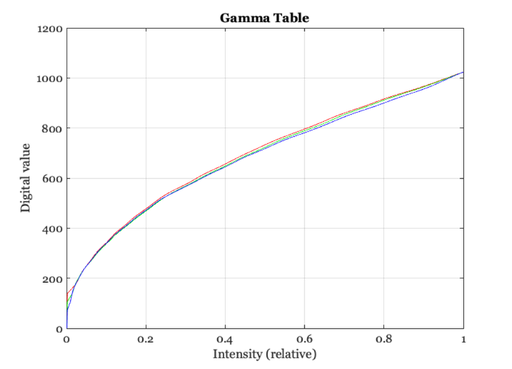
whiteRGB = (xyz2rgb*whiteXYZ)'
whiteMax = max(whiteRGB)

varyRGB = (xyz2rgb*varyXYZ);
varyRGB = varyRGB/whiteMax;

% Use the routine:
invGamTable = displayGet(d,'inverse gamma',1000);
relativeIntensity = (1:length(invGamTable))/length(invGamTable);
whiteRGB =

    1.9997    0.1025    0.6135


whiteMax =

    1.9997
Have a look
vcNewGraphWin;
plot(relativeIntensity,invGamTable)
xlabel('Intensity (relative)'); ylabel('Digital value')
title('Gamma Table');
grid on
Show examples of LAB varying images
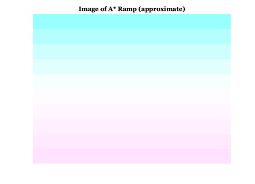
% There are some simple tools for creating images on a standard display
% (sRGB).
%
% First put the varyXYZ (Astar varied) values a 3D array
varyXYZ = ieLAB2XYZ(varyAstarLAB',whiteXYZ)'
fbRGB = xyz2srgb(XW2RGBFormat(varyXYZ',nChips,1))
vcNewGraphWin;
image(fbRGB)
title('Image of A* Ramp (approximate)');
axis off

% Let's make a similar picture as we vary the b* dimension.
% Because we have various bits of information loaded up already
% we can compute a little more quickly.
varyXYZ =

  Columns 1 through 7

   30.0254   31.8227   33.6904   35.6297   37.6421   39.7289   41.8914
   40.7494   40.7494   40.7494   40.7494   40.7494   40.7494   40.7494
   44.2386   44.2386   44.2386   44.2386   44.2386   44.2386   44.2386

  Columns 8 through 10

   44.1310   46.4490   48.8468
   40.7494   40.7494   40.7494
   44.2386   44.2386   44.2386


fbRGB(:,:,1) =

    0.5921
    0.7030
    0.7983
    0.8835
    0.9617
    1.0000
    1.0000
    1.0000
    1.0000
    1.0000


fbRGB(:,:,2) =

    1.0000
    1.0000
    1.0000
    1.0000
    1.0000
    0.9895
    0.9662
    0.9413
    0.9145
    0.8857


fbRGB(:,:,3) =

    0.9931
    0.9942
    0.9954
    0.9965
    0.9977
    0.9990
    1.0000
    1.0000
    1.0000
    1.0000
Create the varyBstar values
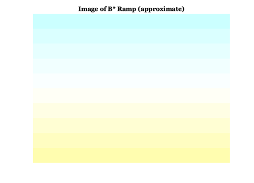
varyBstar(1,:) = 70*ones(1,nChips); % L
varyBstar(2,:) = zeros(1,nChips);   % A*
varyBstar(3,:) = aRamp;             % B*

% Convert Lab to XYZ values
varyXYZ = ieLAB2XYZ(varyBstar',whiteXYZ)'
fbRGB = xyz2srgb(XW2RGBFormat(varyXYZ',nChips,1))
image(fbRGB)
title('Image of B* Ramp (approximate)');
axis off

% By the way: do you see a visual illusion in these images?  The regions
% near the edges (the stimulus is constant) are called colored Mach Bands.
varyXYZ =

  Columns 1 through 7

   38.6761   38.6761   38.6761   38.6761   38.6761   38.6761   38.6761
   40.7494   40.7494   40.7494   40.7494   40.7494   40.7494   40.7494
   76.8896   68.5822   60.8959   53.8064   47.2897   41.3216   35.8781

  Columns 8 through 10

   38.6761   38.6761   38.6761
   40.7494   40.7494   40.7494
   30.9349   26.4680   22.4532


fbRGB(:,:,1) =

    0.7965
    0.8541
    0.9031
    0.9454
    0.9822
    1.0000
    1.0000
    1.0000
    1.0000
    1.0000


fbRGB(:,:,2) =

    1.0000
    1.0000
    1.0000
    1.0000
    1.0000
    0.9993
    0.9968
    0.9946
    0.9925
    0.9907


fbRGB(:,:,3) =

    1.0000
    1.0000
    1.0000
    1.0000
    1.0000
    0.9643
    0.8959
    0.8273
    0.7582
    0.6881
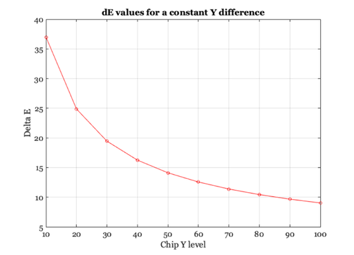
The Delta E_ab value
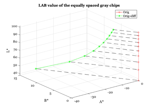
% A central purpose in creating the CIELAB Metric is to be able
% to measure the perceived difference between pairs of lights
% (when the lights are not too dissimilar).

% Create a simple XYZ difference.  Specifically, this difference is 5
% units of Y.  We will add this difference into all of the gray series.
% Notice that we add the same difference to every one of the gray chips.
deltaXYZ = zeros(size(grayXYZ));
deltaXYZ(2,:) = (whiteXYZ(2)/20);
deltaXYZ

% Measure the Lab differences between the original grayXYZ and these
% values with the constant difference (deltaXYZ) added into each gray chip.
%
lab1 = ieXYZ2LAB( grayXYZ.', whiteXYZ.' ).';
lab2 = ieXYZ2LAB( ( grayXYZ + deltaXYZ ).', whiteXYZ.' ).';
diffLAB = lab1 - lab2;

% To see the LAB values in three space for the grayXYZ series and the one
% separated by deltaXYZ, use this code.  It shows the series of LAB values
% of the two different sets, separated by a constant difference.
%
vcNewGraphWin; plot3(lab1(2,:),lab1(3,:),lab1(1,:),'-o',...
    lab2(2,:),lab2(3,:),lab2(1,:),'-*')

for ii=1:size(lab1,2);
    hold on;
    plot3([lab1(2,ii); lab2(2,ii)], ...   % A;egmoqs
        [lab1(3,ii); lab2(3,ii)], ... % B
        [lab1(1,ii); lab2(1,ii)], 'k--'); % L
end
hold off; grid on;
zlabel('L*'), xlabel('A*'); ylabel('B*')
title('LAB value of the equally spaced gray chips')
legend('Orig', 'Orig+diff', 'Location','NorthEast');

% Now we can compute the magnitude of these differences, which is
% called delta Eab.
%
nChips = size(grayXYZ,2)
for i=1:nChips
    dEab(i) = norm( diffLAB(:,i));
end

% Recall that the deltaXYZ is the same at all these levels.  But,
% the delta Eab varies because we are more sensitive at lower
% intensity levels than at high one.  So, the delta Eab value for
% at the dark chips is much larger than the delta Eab value
% for the light chips.
%
% (Note that this is a simplified version of the information
%  in the 3D plot above.)
%
vcNewGraphWin; plot(grayXYZ(2,:),dEab,'-o')
xlabel('Chip Y level'); ylabel('Delta E');
title('dE values for a constant Y difference')
grid on
deltaXYZ =

     0     0     0     0     0     0     0     0     0     0
     5     5     5     5     5     5     5     5     5     5
     0     0     0     0     0     0     0     0     0     0


nChips =

    10
End of tutorial
BEGIN TUTORIAL QUESTIONS --
Question 1: Suppose you had to choose a set of gray reflectances that are equally spaced in LAB coordinates. How would you choose the reflectance levels of the gray series? Explain this qualitatively, based on the CIELAB metric formula (See Color Appearance Lecture Notes).
Question 2: Is visual sensitivity greater for distinguishing the mean reflectance of dark surfaces or light surfaces? Justify your answer using the CIELAB formula. (See Color Appearance Lecture Notes).
Question 3: Suppose we measure the XYZ values of each of a pair of lights. According to the CIELAB metric, what other values must we measure before we can predict the discriminability of these lights? What basic processes in the visual system do these other values represent?
Question 4: Set the white point to whiteXYZ = [100,100,100]; Consider the point pXYZ = [50,100,100]; What is the delta E spacing between pXYZ and another point that differs by 5 units in each principal direction (e.g., [55,100,100])?
Question 5: USING CIELAB TO COMPARE IMAGES
Define the colors yellowRGB = [1.0 1.0 0.0] blueRGB = [0.25 0.625 1.0] greenRGB = [0.625, 0.8125, 0.5]
a) Compute the XYZ values for these colors when displayed on our standard (linear) monitor (i.e., ignore gamma correction).
b) Compute the LAB values for these colors for a white point of whiteXYZ = [95 100 108]
Change the white point to whiteXYZ = [108 100 95] and compute the LAB values again. Does the white point have a big effect? Does changing the white point have the same effect on L, a* and b*?
c) Using the original white point whiteXYZ = [95 100 108], compute the delta E difference between each combination of the three colors (yellowRGB ...). Based on these results, which pair of colors is most dissimilar?
d) Use the following code to generate three images imYB1, imYB2, and imG. (Do not submit these images, but you may describe what you see.)
       imw = 128;
       imYB1 = repmat(reshape(yellowRGB,1,1,3), [256 imw]);
       ss = 1;
       for ii = 1:ss
           imYB1(ii:(2*ss):256, :, :) = ...
               repmat(reshape(blueRGB,1,1,3), [256/ss/2 imw]);
       end
       imYB2 = repmat(reshape(yellowRGB,1,1,3), [256 imw]);
       ss = 16;
       for ii = 1:ss
           imYB2(ii:(2*ss):256, :, :) = ...
               repmat(reshape(blueRGB,1,1,3), [256/ss/2 imw]);
       end
imG = repmat(reshape(greenRGB,1,1,3), [256, imw]);
Measure the delta E difference between imYB1 and imG, and the difference between imYB2 and imG, and compare these values. Define the difference between two images to be the average delta E difference across all pixels. (Use the white point whiteXYZ = [95 100 108]).
Hints: - You may find the command imdata = reshape(im, size(im,1)*size(im,2),3); useful for transforming an m x n x 3 image into an (m*n) x 3 matrix of pixels.
- You can use ieXYZ2LAB to convert XYZ data to LAB data in bulk. ieXYZ2LAB may take an nx3 matrix of XYZ values to LAB values (where each row is an XYZ color vector).
e) View the images side by side and compare them. Notice that the average delta E of (imYB1 vs imG) and of (imYB2 vs imG) do not agree with the appearance similarity. Explain why you think the appearance and delta E values diverge. Suggest a way to improve the CIELAB metric so it more accurately reflects the perceived difference.