Barten's SQRI metrics

Calculate the SQRI metric (The Square Root Integral (SQRI): A New Metric To Describe The Effect Of Various Display Parameters On Perceived Image Quality)

Invented in 1989 by Barten in an SPIE paper.

For the calculation here, notice when the display MTF is all ones, we achieve the highest level of SQRI we could obtain for a human in that viewing condition (which depends on the luminance and width parameters, L and w).

Spatial frequency

nSF = 5000;                    % For the integration to go well, 5K samples
sf = logspace(-1.5,1.6,nSF);   % Spatial frequency values
dMTF = ones(size(sf));         % Put in a perfect display to start
L = 340/pi;                    % Luminance in cd/m2
widths = [0.5 1 2.3 6.5 60];   % Deg of visual angle for the display

Match Figure 2 theoretical curves of CSF

% Barten calls 1/Mt the CSF
hCSF = zeros(length(sf),length(widths));
lText = cell(1,length(widths));
for ll = 1:length(widths)
    [maxSQRI, hCSF(:,ll)] = ieSQRI(sf, dMTF, L, 'width',widths(ll));
    lText{ll} = sprintf('W=%.1f\n',widths(ll));
end
vcNewGraphWin;
loglog(sf,hCSF)
xlabel('Spatial Frequency (cpd)');
ylabel('Sensitivity (1/thresh)');
set(gca,'xlim',[0.01,100],'ylim',[1 1000]); grid on
legend(lText)
fprintf('Max SQRI %.3f  (L = %f, width = %f)\n',maxSQRI,L, widths(end));

Max SQRI 143.412  (L = 108.225361, width = 60.000000)

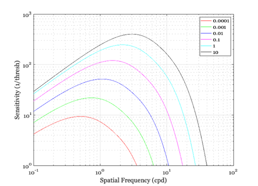
Figure 3

% Barten calls 1/Mt the CSF
Ls = logspace(-4,1,6);
hCSF = zeros(length(sf),length(Ls));
lText = cell(1,length(Ls));
width = 14;
for ll = 1:length(Ls)
    [maxSQRI, hCSF(:,ll)] = ieSQRI(sf, dMTF, Ls(ll), 'width',width);
    lText{ll} = sprintf('%g\n',Ls(ll));
end

vcNewGraphWin;
loglog(sf,hCSF)
xlabel('Spatial Frequency (cpd)');
ylabel('Sensitivity (1/thresh)');
set(gca,'xlim',[0.1,100],'ylim',[1 1000]); grid on
legend(lText)

fprintf('Max SQRI %.3f  (L = %f, width = %f)\n',maxSQRI,L, width);

Max SQRI 111.019  (L = 108.225361, width = 14.000000)

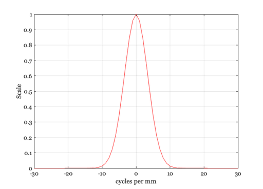
Now, we make a display MTF and do the same calculation

% A display MTF might be calculated from the display pointspread, say given
% in units of cycles/meter and then converted to cycles per degree by
% knowing the user's viewing distance.

% Suppose we treat the display pixel as a Gaussian whose standard deviation
% extends to the edge of the pixel, so that each pixel width is 2 sigma
d = displayCreate('OLED-Samsung-Note3');
sigma = 0.5*displayGet(d,'meters per dot','um');

% This produces a symmetric Gaussian with a peak at f=x=0
x = -500:499;             % 1000 um steps, 1 mm total
g = exp(-(x/sigma).^2);   % Gaussian in um steps
g = g/sum(g(:));          % Force to unit area so DC is 1

dMTF = fftshift(abs(fft(g)));
fcpmm = x;       % cycles per mm because 1 cycle is 1 mm wavelength
vcNewGraphWin; plot(fcpmm,dMTF); set(gca,'xlim',[-30 30])
xlabel('cycles per mm'); ylabel('Scale'); grid on

Now convert to cycles per deg from cycles per mm

% This depends on viewing distance
vDist = [0.2 0.4 0.8];  % Meters
vcNewGraphWin;
for vv = 1:length(vDist)
    % We need the scalar of (mm/deg)
    % So we can calculate cyc/deg = cyc/mm * (mm/deg)
    d = displaySet(d,'viewing distance',vDist(vv));
    mmPerDeg = displayGet(d,'dots per deg')*displayGet(d,'meters per dot','mm');
    fcpd = fcpmm*mmPerDeg;
    % Show the display MTF in cyc/deg
    plot(fcpd,dMTF); hold on;
end
xlabel('cpd')
ylabel('Scale')
set(gca,'xlim',[-60 60])

So, let's compute with everything we need in one cell

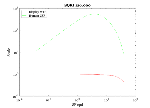
% This is a high resolution display:   dName = 'OLED-Samsung-Note3';
% This is a modest resolution display:
dName = 'CRT-HP';
d = displayCreate(dName);

% Here is the display viewing distance and dpi
vDist = 1;
d = displaySet(d,'viewing distance',vDist);
sigma = 0.5*displayGet(d,'meters per dot','um');

% Calculate the dMTF
% This produces a symmetric Gaussian with a peak at f=x=0
x = -500:499;             % 1000 um steps, 1 mm total
g = exp(-(x/sigma).^2);   % Gaussian in um steps
g = g/sum(g(:));          % Force to unit area so DC is 1
dMTF = fftshift(abs(fft(g)));

fcpmm = x;       % cycles per mm because 1 cycle is 1 mm wavelength
mmPerDeg = displayGet(d,'dots per deg')*displayGet(d,'meters per dot','mm');
fcpd = fcpmm*mmPerDeg;

% Interpolate to
% sf = linspace(0,100,100);
sf = logspace(-1.5,1.6,nSF);
dMTF = interp1(fcpd,dMTF,sf);
% vcNewGraphWin; plot(sf,dMTF);

L     = 100;    % cd/m2;
width = 14;     % Deg
[sqri, CSF] = ieSQRI(sf, dMTF, L, 'width',width);
fprintf('%s: dpi = %.1f   SQRI %.1f  L %.1f Width %.1f nSF %d\n',dName, displayGet(d,'dpi'),sqri, L, width, nSF);

CRT-HP: dpi = 96.0   SQRI 126.0  L 100.0 Width 14.0 nSF 5000

How to interpret the numbers and values?

Barten 1990 Figure 7 plots SQRI values around 100 for their older displays. The numbers we compute here seem similar.

We should check the Korean 2010 paper, as well. More replications and testing of published material.

vcNewGraphWin; loglog(sf,dMTF,'r-',sf,CSF,'g--');
legend({'Display MTF','Human CSF'},'location','NorthWest')
xlabel('SF cpd');
ylabel('Scale');
title(sprintf('SQRI %.3f',sqri));

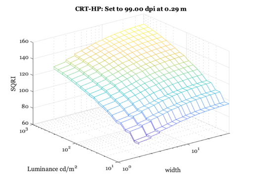
We might make a SQRI surface with (width,L) as parameters

% The basic calculation depends only on
% * dpi, L, width, vDist
%
% So we can fix any two of them and show a surface for the other
% two. Some of these surfaces correspond to the values in the
% 1989 publication cited above.

L     = logspace(1,3,20);
vDist = logspace(-0.7,0,10);
width = round(logspace(0.3,1.6,20));
dpi   = round(linspace(70,200,10));

% This is a high resolution display:   dName = 'OLED-Samsung-Note3';
% This is a modest resolution display:
dName = 'CRT-HP';
d = displayCreate(dName);

% Create the dMTF
vDistIdx = 3;
dpiIdx   = 3;
d = displaySet(d,'viewing distance',vDist(vDistIdx));
d = displaySet(d,'viewing distance',dpi(dpiIdx));

% Here is the display viewing distance and dpi
sigma = 0.5*displayGet(d,'meters per dot','um');

% Calculate the dMTF
% This produces a symmetric Gaussian with a peak at f=x=0
x = -500:499;             % 1000 um steps, 1 mm total
g = exp(-(x/sigma).^2);   % Gaussian in um steps
g = g/sum(g(:));          % Force to unit area so DC is 1
dMTF = fftshift(abs(fft(g)));

fcpmm = x;       % cycles per mm because 1 cycle is 1 mm wavelength
mmPerDeg = displayGet(d,'dots per deg')*displayGet(d,'meters per dot','mm');
fcpd = fcpmm*mmPerDeg;

% Interpolate to
% sf = linspace(0,100,nSF);
sf = logspace(-1.5,1.6,nSF);
dMTF = interp1(fcpd,dMTF,sf);

% Loop on width and luminance
sqri = zeros(length(width),length(L));
for ww=1:length(width)
    for ll = 1:length(L)
        sqri(ww,ll) = ieSQRI(sf, dMTF, L(ll), 'width',width(ww));
    end
end

vcNewGraphWin; mesh(width,L,sqri);
set(gca,'xscale','log','yscale','log');
xlabel('width'); ylabel('Luminance cd/m^2'); zlabel('SQRI')
title(sprintf('%s: Set to %.2f dpi at %.2f m',dName, dpi(dpiIdx), vDist(vDistIdx)));