Evaluating an infrared camera MTF
Calculate the ISO12233 MTF the slanted edge target.
This is a long (and older) version of the more calculation illustrated in s_metricsMTFSlantedBar.
The processing steps illustrated are
- Create a slanted bar scene with infrared data
- Convert the scene to an optical image
- Create a sensor with 7 bands and a random spatial CFA and compute the virtual camera image
- Interactively select the rectangular region and store it
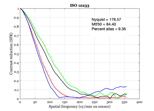
- Compute the MTF of the slanted edge target for this sensor and spatial CFA
See also: sceneCreate, ieReadColorFilter, ieRect2Locs, vcGetROIData, ISO12233
Copyright ImagEval Consultants, LLC, 2010
Contents
- First, create a slanted bar image. Make the slope some uneven value
- Create an optical image with some default optics.
- Create sensor
- Create and set the processor window
- Define the rect for the ISO12233 calculation
- Calculate an MTF when you choose the rectangle
- Compare what happens when we place an IR blocking filter in the path
- Compute the MTF with the rectangle selected automatically
- END
ieInit
First, create a slanted bar image. Make the slope some uneven value
sz = 512;    %Row and col samples
slope = 7/3;
meanL = 100; % cd/m2
viewD = 1;   % Viewing distance (m)
fov   = 5;   % Horizontal field of view  (deg)
wave = 400:4:1068;

scene = sceneCreate('slantedBar',sz,slope,fov,wave);

% Now we will set the parameters of these various objects.
% First, let's set the scene field of view.
scene = sceneAdjustLuminance(scene,meanL);    % Candelas/m2
scene = sceneSet(scene,'distance',viewD);     % meters
scene = sceneSet(scene,'fov',fov);            % Field of view in degrees

% sceneWindow(scene);
Create an optical image with some default optics.
oi = oiCreate('diffraction limited');
fNumber = 4;
oi = oiSet(oi,'optics fnumber',fNumber);

% Now, compute the optical image from this scene and the current optical
% image properties
oi = oiCompute(oi,scene);
% oiWindow(oi);
Create sensor
% Build a default sensor
sensor = sensorCreate;
wave   = sceneGet(scene,'wave');
[filterSpectra,allNames] = ieReadColorFilter(wave,'NikonD200IR.mat');

% This is a way to make artificial color filters, each with a Gaussian
% sensitivity profile.
%    nSensors = 7; minW = 450; maxW = 800;
%    cPos = linspace(minW,maxW,nSensors);
%    width = ones(size(cPos))*(cPos(2)-cPos(1))/2; cfType = 'gaussian';
%    filterSpectra = sensorColorFilter(cfType, wave, cPos, width);
%    allNames = {'b1','g1','r1','x1','i1','z1','i2'};

% Spatial layout is 3x3 for seven sensor case.
%    p = [ 1 2 3; 4 5 6; 7 7 7];
%    sensor = sensorSet(sensor,'pattern and size',p);
%    sensorShowCFA(sensor);

nSensors    = length(allNames);
filterNames = cell(1,nSensors);
for ii=1:nSensors, filterNames{ii} = allNames{ii}; end
% ieNewGraphWin; plot(wave,filterSpectra)

% Adjusting the wavelength requires updating several fields - the
% sensor, the pixel, the photodetector QE, and the infrared
% filter.  The pixel wave is updated automatically, but it is
% necessary to also update the infrared and photodetector QE -
sensor = sensorSet(sensor,'wave',wave);
sensor = sensorSet(sensor,'filterSpectra',filterSpectra);
sensor = sensorSet(sensor,'filterNames',filterNames);
sensor = sensorSet(sensor,'ir filter',ones(size(wave)));
% ieNewGraphWin; plot(wave,sensorGet(sensor,'irFilter'))

pixel  = sensorGet(sensor,'pixel');
pixel  = pixelSet(pixel,'pd spectral qe',ones(size(wave)));
sensor = sensorSet(sensor,'pixel',pixel);
% ieNewGraphWin; plot(wave,pixelGet(pixel,'pd spectral qe'))

% Match the sensor size to the scene FOV. Also matches the CFA size to the
% sensor (I think).
sensor = sensorSetSizeToFOV(sensor,sceneGet(scene,'fov'),oi);

% Compute the image and bring it up.
sensor = sensorCompute(sensor,oi);
% sensorWindow(sensor);

% Plot a couple of lines
%    sensorPlotLine(sensor,'h','volts','space',[1,80]);
%    sensorPlotLine(sensor,'h','volts','space',[1,81]);
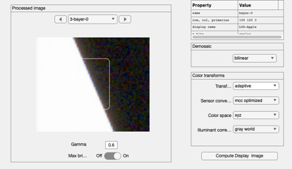
Create and set the processor window
ip = ipCreate;
ip = ipSet(ip,'scale display',1);
ip = ipSet(ip,'render Gamma',0.6);

% Use the linear transformation derived from sensor space (above) to
% display the RGB image in the processor window.
ip = ipSet(ip,'conversion method sensor ','MCC Optimized');
ip = ipSet(ip,'correction method illuminant ','Gray World');%
ip = ipSet(ip,'internal CS','XYZ');

% First, compute with the default properties.  This uses bilinear
% demosaicing, no color conversion or balancing.  The sensor RGB
% values are simply set to the display RGB values.
ip = ipCompute(ip,sensor);
ipWindow(ip);
Define the rect for the ISO12233 calculation
% Have the user select the edge.
masterRect = [39    25    51    65];

% This changed around December 2023.  Not sure why.  Probably some
% object changed size? (BW)
% Then it changed back.
% masterRect = [166    82   226   303];

% It is also possible to estimate the rectangle automatically using
% ISOFindSlantedBar, which is called in ieISO12233()
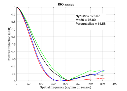
Calculate an MTF when you choose the rectangle
roiLocs = ieRect2Locs(masterRect);

% BUG HERE
barImage = vcGetROIData(ip,roiLocs,'results');
c = masterRect(3)+1;
r = masterRect(4)+1;
barImage = reshape(barImage,r,c,3);
%{
ieNewGraphWin;
imagesc(barImage(:,:,1));
axis image; colormap(gray(64));
%}

dxmm = sensorGet(sensor,'pixel width','mm');

% Run the ISO 12233 code.  The results are stored in the window.
ISO12233(barImage, dxmm);
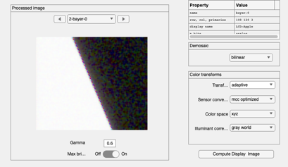
Compare what happens when we place an IR blocking filter in the path
[irFilter,irName] = ieReadColorFilter(wave,'IRBlocking');
% ieNewGraphWin; plot(wave,irFilter);

sensor = sensorSet(sensor,'ir filter',irFilter);
sensor = sensorCompute(sensor,oi);
ieAddObject(sensor);
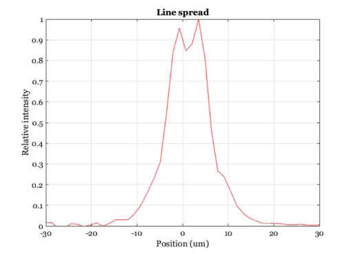
Compute the MTF with the rectangle selected automatically
ip = ipCompute(ip,sensor);

% Compute the MTF and the Linespread function
mtf = ieISO12233(ip);

ieNewGraphWin;
mtf.lsfx = mtf.lsfx*1000;  % Convert to microns
plot(mtf.lsfx, mtf.lsf);
xlabel('Position (um)'); ylabel('Relative intensity');
title('Line spread'); grid on;
dxum = dxmm*1000;
mxmn = 30;
set(gca,'xlim',[-mxmn mxmn],'ylim',[0 1]);

% Inserted 2023.12.28
assert(abs(mtf.mtf50 - 77) <= 3);

ipWindow(ip);
h = ieDrawShape(ip,'rectangle',mtf.rect);
Using selected sensor
No black border detected