Use the edge of the slanted bar to estimate the MTF

The ISO 12233 standard defines a modulation transfer function for assessing system acuity. We calculate the MTF (also called the spatial frequency response, or sfr, in the color literature).

This script also illustrates how to

define a scene
create an optical image from the scene
define a monochrome sensor
evaluate the sensor MTF

We measure the system MTF properties using a simple slanted bar target along with the ISO 12233 standard methods.

This script is an example of a complicated (but useful) calculation. We suggest that you begin programming scripts using other, simpler routines. We include this script because it shows many features of the scripting language and the ability to interact with the GUI from scripts.

See also: sensorCompute, sensorCreate, s_pixelSizeMTF, ISOFindSlantedBar, ipCompute, ipCreate,

First, create a slanted bar image. Make the slope some uneven value
Create an optical image with some default optics.
Create a default monochrome image sensor array
Run the computation for the monochrome sensor
Slide into agreement in space, then FFT
Here is the MTF of the mean

ieInit

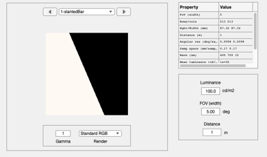
First, create a slanted bar image. Make the slope some uneven value

sz = 512;    % Row and col samples
slope = 7/3;
meanL = 100; % cd/m2
viewD = 1;   % Viewing distance (m)
fov   = 5;   % Horizontal field of view  (deg)

scene = sceneCreate('slantedBar',sz,slope);

% Now we will set the parameters of these various objects.
% First, let's set the scene field of view.
scene = sceneAdjustLuminance(scene,meanL);    % Candelas/m2
scene = sceneSet(scene,'distance',viewD);       % meters
scene = sceneSet(scene,'fov',fov);            % Field of view in degrees
ieAddObject(scene); sceneWindow;

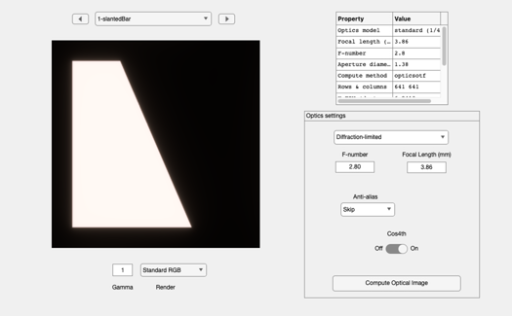
Create an optical image with some default optics.

oi = oiCreate;

fNumber = 2.8;
oi = oiSet(oi,'optics fnumber',fNumber);

% Now, compute the optical image from this scene and the current
% optical image properties
oi = oiCompute(oi,scene);
ieAddObject(oi); oiWindow;

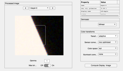
Create a default monochrome image sensor array

sensor = sensorCreate;                 % RGB sensor

sensor = sensorSet(sensor,'autoExposure',1);
sensor = sensorCompute(sensor,oi);

Run the computation for the monochrome sensor

ip = ipCreate;
ip = ipCompute(ip,sensor);
ieAddObject(ip); ipWindow;

Find a good rectangle

masterRect = ISOFindSlantedBar(ip);
h = ieDrawShape(ip,'rectangle',masterRect);

barImage = vcGetROIData(ip,masterRect,'results');
c = masterRect(3)+1;
r = masterRect(4)+1;
barImage = reshape(barImage,r,c,3);

vcNewGraphWin; imagesc(barImage(:,:,1)); axis image; colormap(gray(64));
for ii=1:r
    plot(barImage(ii,:,1));
    hold on;
end

No black border detected

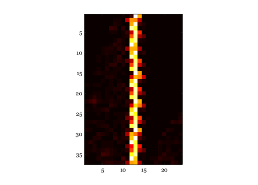
Slide into agreement in space, then FFT

% Pull out the green channel
img = barImage(:,:,2);
dimg = diff(img,1,2);
dimg = abs(dimg);

vcNewGraphWin; imagesc(dimg); axis image; colormap(hot(64))
col = size(dimg,2);
row = size(dimg,1);
dimgS = zeros(size(dimg));

% We could align them in a better way!
fixed = dimg(20,:);
for rr = 1:row
    [c,lags] = ieCXcorr(fixed,dimg(rr,:));
    % vcNewGraphWin; plot(1:col,fixed,'o-',1:col,dimg(rr,:),'x-');
    [~,ii] = max(c);
    dimgS(rr,:) = circshift(dimg(rr,:)',lags(ii))';
end
vcNewGraphWin; imagesc(dimgS); axis image; colormap(hot(64))

% Here is the mean after aligning
mn = mean(dimgS);
% Make this have unit area
mn = mn / sum(mn);
vcNewGraphWin; plot(mn)

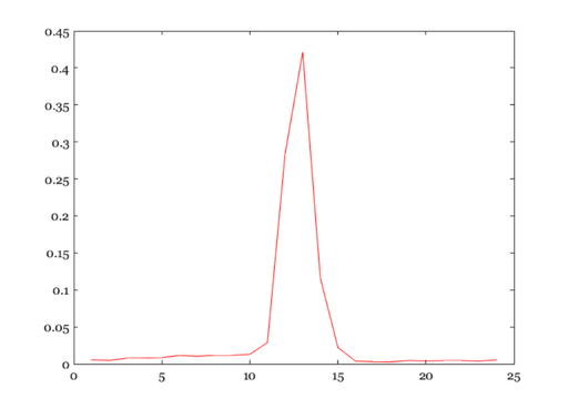
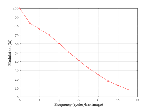
Here is the MTF of the mean

mtf = abs(fft(mn));
freq = (1:round((col/2))) - 1;
vcNewGraphWin; plot(freq,100*mtf(1:length(freq)),'o-')
xlabel('Frequency (cycles/bar image)')
ylabel('Modulation (%)')
grid on