JPEG color compression review

AUTHOR:   X. Zhang, B. Wandell
PURPOSE:  Develop JPEG compression in color
DATE:     02.15.96

We integrate the basic DCT calculations with color transformations. We introduce YCbCr and some additional discussion of chrominance subsampling and color lookup tables. Finally, we try a simple experiment with jpeg compression by switching the luminance and chrominance quantization tables.

Matlab 5: Checked 01.06.98, BW Matlab 7: Checked 01.02.08 BW

JPEG compression of color image
JPEG Color spaces: YCbCr
BEGIN TUTORIAL QUESTIONS

ieInit

JPEG compression of color image

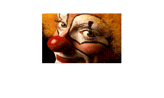
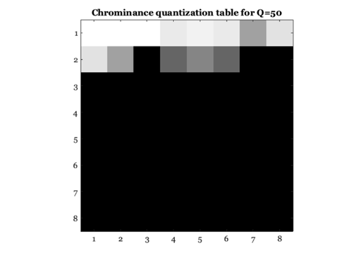
% Load in a color image.  This is an indexed color image.

D = load('jpegFiles/clown.mat');
map = D.map;
img = D.X;
vcNewGraphWin;
imshow(img, map);

% Convert the image into RGB format.
%
[r,g,b] = ind2rgb(img, map);

% Recall that JPEG works on each color plane separately.  Hence,
% in principle it is possible to apply JPEG to each of these
% three color planes separately.
%
qFactor = 75;
rCoef = jpegCoef(r,qFactor);
gCoef = jpegCoef(g,qFactor);
bCoef = jpegCoef(b,qFactor);

% You can see that we did well in terms of zeroing lots of the
% coefficients so that the result will be strongly compressed.
%
histogram(bCoef(:),[-100:10:260])
title('Histogram of quantized coefficients (b channel)');

% To prove this, let's just consider some of the sizes of things.
% This isn't exactly fair or precise, but we can get a rough idea
% of how compressible the different image data sets are by
% writing them out as matlab files and then measuring their entropy, or
% just by trying to compress them.

% (technical note: -v4 forces Matlab to save with no compression and
%  not to optimize by changing to a lower-precision data type even
%  if possible.)

save -v4 rgbImage r g b;
save -v4 dctCoef rCoef gCoef bCoef;

% We now measure the mathematical entropy of each file.  Entropy can be
% interpreted as a measure of the theoretical limit on the compressibility
% of data.  A lower entropy means that the data is more compressible.

rgbEntropy = entropy_file('rgbImage.mat')
dctEntropy = entropy_file('dctCoef.mat')

% If you're not convinced, or you're not familiar with entropy, You might
% also try running these commands, which, in Matlab v7, saves the
% data in a (lossless) compressed format to see how compressible the data
% is.
% save rgbImageComp r g b;
% save dctCoefComp  rCoef gCoef bCoef;


% Clean up and go back
%
unix('rm -f dctCoef* rgbImage*');

% Now, we will invert the coefficients and see what the image
% looks like.
rJPEG = truncate(jpegRGB(rCoef,qFactor),0,255);
gJPEG = truncate(jpegRGB(gCoef,qFactor),0,255);
bJPEG = truncate(jpegRGB(bCoef,qFactor),0,255);

% foo = jpegRGB(rCoef,q1); histogram(foo(:))
% histogram(rJPEG(:))
Xjpeg(:,:,1) = rJPEG; Xjpeg(:,:,2) = gJPEG; Xjpeg(:,:,3) = bJPEG;
imshow(Xjpeg/255);

% In the JPEG_bw tutorial, we showed you the quantization tables for the
% luminance plane.  In addition to the quantization matrices for the
% luminance plane, there there is also a quantization matrix for the
% chrominance plane.  As you can see, the standard chrominance table is
% very coarse for color.

% For these pictures of the quantization table, lighter means that the
% coefficients will be better preserved, and dark means that the
% coefficients will be more highly quantized.

Q_factor = 50;
q2 = jpeg_qtables(Q_factor,2)
vcNewGraphWin;
colormap(gray(64));
imagesc(256 - q2), axis image
title(sprintf('Chrominance quantization table for Q=%d',Q_factor));

% Again, if you want to know how the scaling of quantization tables was
% done, look at the code in jpeg_qtables.
%
% type jpeg_qtables

jpegCoef:  Using passed quality factor
Image max < 1.  Treating as 8 bit input
jpegCoef:  Using passed quality factor
Image max < 1.  Treating as 8 bit input
jpegCoef:  Using passed quality factor
Image max < 1.  Treating as 8 bit input

rgbEntropy =

    1.4065


dctEntropy =

    0.6140


q2 =

    17    18    18    24    21    24    47    26
    26    47    99    66    56    66    99    99
    99    99    99    99    99    99    99    99
    99    99    99    99    99    99    99    99
    99    99    99    99    99    99    99    99
    99    99    99    99    99    99    99    99
    99    99    99    99    99    99    99    99
    99    99    99    99    99    99    99    99

JPEG Color spaces: YCbCr

% Because the eye is insensitive to fine chromatic contrasts, we
% can compress the chromatic components of an image more than the
% light-dark component without much change in the image quality.
% In JPEG this is accomplished by transforming the RGB signals
% into a new color representation, commonly called Y,Cb,Cr, and
% then compressing the chromatic components (Cb,Cr) more than the
% luminance component (Y).

% In principle, you  might imagine that the standard would take
% into account the actual display you are using.  But, no.  Also,
% in principle, you would imagine that the standard might work in
% a space that reflected light intensity rather than frame
% buffers.  But, no.

% Rather, the transformation from RGB to YCbCr is hardcoded into
% a matrix

RGB2YCC = ...
    [ 0.2990 0.5870  0.1140; ...
    -0.1687 -0.3313 0.5000; ...
    0.5000 -0.4187 -0.0813]

% To apply this transformation to the r,g,b image data we do
%
Y =   0.2990*r + 0.5870*g + 0.1140*b;
Cb = -0.1687*r - 0.3313*g + 0.5000*b;
Cr =  0.5000*r - 0.4187*g - 0.0813*b;

% Now, we compute the coefficients of the Y image using a
% different quantization table from the Cb and Cr images.  In
% fact, the JPEG-DCT has two default quantization tables: one for
% the luminance component (Y),
qFactor = 75;
q1 = jpeg_qtables(qFactor, 1)

% and the other for the chrominance components (Cb, Cr).
%
q2 = jpeg_qtables(qFactor, 2)

% In general, the chrominance quantization table has larger
% quantization steps sizes than the luminance one.  Also, it is
% applied to THE SUBSAMPLED chrominance bands.  This saves a
% great deal of space.  At this moment, this is not implemented
% in this tutorial, so we will simply use

q2 = q1;

% Now we compress the clown image using these quantization
% tables.
Ycoef  = jpegCoef(Y, q1);
Cbcoef = jpegCoef(Cb,q2);
Crcoef = jpegCoef(Cr,q2);

% histogram(Ycoef(:),[-100:10:200])
% histogram(Cbcoef(:),[-100:10:200])

yJPEG   = jpegRGB(Ycoef,q1);
CbJPEG  = jpegRGB(Cbcoef,q2);
CrJPEG  = jpegRGB(Crcoef,q2);

% histogram(yJPEG(:))

% Convert the compressed YCbCr image back into RGB format
rJPEG = truncate(yJPEG + 1.4020*CrJPEG,0,255);
gJPEG = truncate(yJPEG - 0.3441*CbJPEG - 0.7141*CrJPEG,0,255);
bJPEG = truncate(yJPEG + 1.7720*CbJPEG - 0.0001*CrJPEG,0,255);

% histogram(rJPEG(:),[-100:5:200])
Xjpeg(:,:,1) = rJPEG; Xjpeg(:,:,2) = gJPEG; Xjpeg(:,:,3) = bJPEG;
vcNewGraphWin; imshow(Xjpeg/255);

% Remember: In the usual JPEG implementation, the chromatic
% planes (Cb,Cr) are subsampled by a factor of 2 before applying
% the DCT.  This reduces the representation allocated to the
% chromatic planes and saves lots more space.  It also changes
% the meaning of the spatial frequencies in the q2 quantization
% table.  All of this should be implemented as part of this
% tutorial some day.

RGB2YCC =

    0.2990    0.5870    0.1140
   -0.1687   -0.3313    0.5000
    0.5000   -0.4187   -0.0813


q1 =

     8     6     6     7     6     5     8     7
     7     7     9     9     8    10    12    20
    13    12    11    11    12    25    18    19
    15    20    29    26    31    30    29    26
    28    28    32    36    46    39    32    34
    44    35    28    28    40    55    41    44
    48    49    52    52    52    31    39    57
    61    56    50    60    46    51    52    50


q2 =

     9     9     9    12    11    12    24    13
    13    24    50    33    28    33    50    50
    50    50    50    50    50    50    50    50
    50    50    50    50    50    50    50    50
    50    50    50    50    50    50    50    50
    50    50    50    50    50    50    50    50
    50    50    50    50    50    50    50    50
    50    50    50    50    50    50    50    50

jpegCoef:  Using passed lookup table
Image max < 1.  Treating as 8 bit input
jpegCoef:  Using passed lookup table
Image max < 1.  Treating as 8 bit input
jpegCoef:  Using passed lookup table
Image max < 1.  Treating as 8 bit input

BEGIN TUTORIAL QUESTIONS

1) Describe the information content of each channel of the YCbCr color space, in terms of what image properties the channels convey.

2) What property of color visual sensitivity makes it possible to obtain the high compression ratio if we accept lossy compression? How does the YCbCr color space take advantage of this visual system property?

3) Explore the visual impact of compressing color images in different spaces. Specifically, load a color image into R,G and B planes. Then make a version of the image in YCbCr space, using the linear transformation above.

a)  Use the code from the tutorial to create a very aggressive
quantization table. Use this table and compress the blue channel a lot.
Then show the RGB image with the compressed blue channel.  (Quantize
the other two channels with a q factor of 75.)

Reconstruct and show the result.  Describe what you see.

b) Use the same quantization tables to aggressively compress the Cb
channel.  Reconstruct the image as in the tutorial, and show it. Which
image looks better?  (Quantize the other two channels with a q factor
of 75.)

Reconstruct and show the results.  Describe what you see.

c) To see what the different channels look like, try reconstructing
an image with the CbJPEG set to zero.  Then try it with the CrJPEG set
to zero.  Then try setting the Y channel to all values of 128.  This
is a picture with no luminance, only chrominance.

Bonus Question:

In the Color Matching tutorial, we investigated the implications of
adding a fourth phosphor (ie, channel) to our color monitor.

Assume that the JPEG color gamut is a smaller subset of the visible
gamut, and that the gamut of the three-primary monitor is itself a
smaller subset of the JPEG gamut.

In the color matching tutorial, we noted that the the fourth monitor
primary allowed us to cover a larger area of the visible gamut.
a) Does the fourth primary help in the display of the JPEG image?

b) How would you modify JPEG to take full advantage of the new primary?
Describe how your modification helps, and also any extra data costs.
(Extra bonus: modify the standard without any extra data costs)

JPEG color compression review

Contents

JPEG compression of color image

JPEG Color spaces: YCbCr

BEGIN TUTORIAL QUESTIONS