Introduction to JPEG compression, monochrome case.
  AUTHOR:   X. Zhang, B. Wandell
  PURPOSE:  Explain the basic features of JPEG compression
  DATE:     02.15.96
This tutorial covers the DCT calculation, the dct coefficient quantization, and the inversion process. We will also cover some issues relating to compression of indexed color images.
Matlab 5: Checked 01.06.98, BW Matlab 7: Checked 01.02.08 BW
Contents
ieInit
JPEG compression of a grayscale image
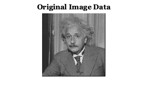
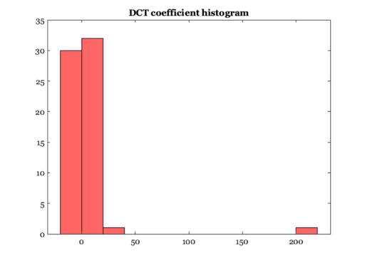
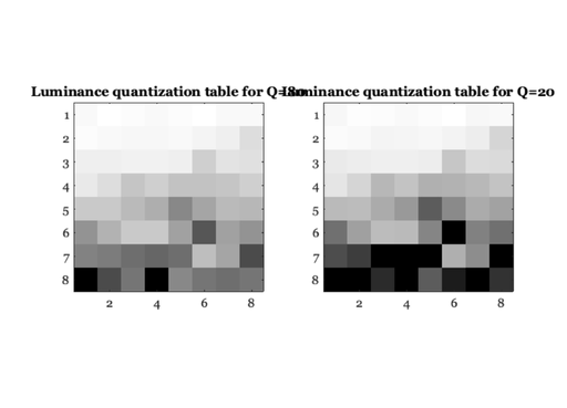
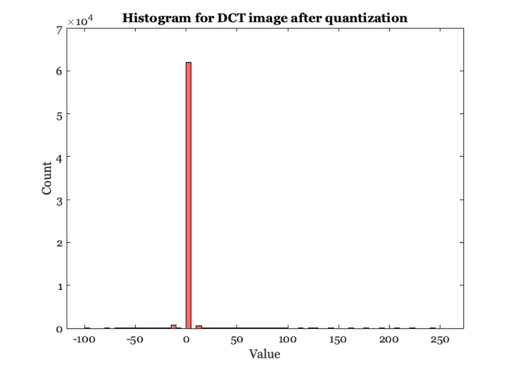
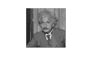
% Let's read in a picture to get started
%
D = load('jpegFiles/einstein.mat');
im = D.X;   % Read in as the variable X
vcNewGraphWin;
imshow(im,[1,256])
title('Original Image Data');

% We are ready to start the compression operations.

% 1.  THE DCT STEP
%
% The first step is dividing the image into little 8x8 blocks,
% and then apply the DCT transformation on each block.  The image
% size is 256x256, these are multiples of 8, so we are in good
% shape.  If we had not had a multiple of 8, then we would have
% taken the last, incomplete block and padded it with zeros.

% To understand the calculation we will first trace what happens
% to a single block. Here is an 8x8 block from the image

block = im(89:96, 105:112)
vcNewGraphWin; histogram(block(:))
title('Histogram of 8x8 block near image center');
xlabel('Pixel value');
ylabel('Count');

% To transform the data in the block, we need to multiply them by
% the cos(x)cos(y) functions of the DCT.  I have stored these
% functions in a file that we can load.  To see how these
% functions are built use
% typejpegFiles/makeDctMatrix.m

load jpegFiles/dctMatrix;

% Each column of this matrix is a cos function at a different
% spatial frequency.  But they are very coarsely sampled and so
% they don't really look familiar.
%
plot(1:size(dctMatrix,1),dctMatrix(:,[1 3 5 7]))
title('Selected DCT basis functions');

% The DCT is separable, so to obtain the dct coefficients for
% this block we can perform a fairly simple matrix multiplication.
% We multiply the columns of the block by the dctMatrix and then
% we multiply the rows.
dctCoef = dctMatrix*block*dctMatrix';
histogram(dctCoef(:))
title('DCT coefficient histogram')

% Here is an image of the coefficients.  We use a nonlinear map
% so that the appearance of the blocks will correspond a little
% better with their actual values.
linMap = gray(256).^0.45;
vcNewGraphWin; colormap(linMap); imagesc(dctCoef);
title('DCT-transformed image data');

% Gray values represent coefficients near zero.  Bright values
% (upper left, the mean) are positive and black values are
% negative.  Notice that the higher order coefficients (lower
% right) are small. They tend to be small in general.

% If we use the DCT function in Matlab to do it, the results are
% the same, except for some extra scaling that is required for
% the JPEG standard.
%
% c = [ 1/sqrt(2) 1 1 1 1 1 1 1 ];
% dctCoef1 = dct(block)'*diag(c)/8;      % apply dct on columns
% dctCoefm = dct(dctCoef1)'*diag(c)/8;   % apply dct on rows
%
% max(abs(dctCoefm(:) - dctCoef(:)))     % results are the same

%%THE QUANTIZATION STEP.
%
% We started with 64 numbers and we still have 64 numbers.  We
% are ready to save information by the quantization step. To
% quantize the dct coefficients, we divide each DCT coefficient
% by its quantization step size, round the result, and then
% multiply with the quantization step size.

% There is a standard quantization table provided by the JPEG
% people.  The one that is hard coded into the C-code is returned
% when you set the quality factor equal to 50.
Q_factor = 50;
q1 = jpeg_qtables(Q_factor,1)

% Big numbers in this table are places where the dct coefficients
% will be strongly quantized.  Small numbers, at the low
% frequency coefficients, will not be quantized as much.
% Notice, that with this default everything is quantized a
% little.  If we want a really high quality factor, look at what
% happens to the table.  Compare it with the previous one.
Q_factor = 90;
q1 = jpeg_qtables(Q_factor,1)

% To make the picture of the quantization table, I have made
% light mean preserve the coefficient and black mean lose it
colormap(linMap);

Q_factor = 80;
subplot(1,2,1); imagesc(256 -jpeg_qtables(Q_factor,1));
title(sprintf('Luminance quantization table for Q=%d',Q_factor));
axis image

Q_factor = 20;
subplot(1,2,2); imagesc(256 - jpeg_qtables(Q_factor,1));
title(sprintf('Luminance quantization table for Q=%d',Q_factor));
axis image

% Now we use the quantization table q1 to quantize the dct
% coefficients for the image block.
% First divide the coefficients by the quantization step size,
% then round, then multiply it back in.

dctQuant = round(dctCoef ./ q1) .* q1

% Notice, there are a lot of zeros in the quantized coefficient
% matrix.  This is good for the lossless compression stage that follows.

% The difference between the original dct coefficient and the
% quantized coefficient will not be larger than quantization step
% size.  We can check this as follows.
%
round(abs(dctQuant - dctCoef))


% Now we will transform-quantize over every block in the image.
% We always work with even blocks, but if the size of the image
% doesn't fill up a block at the edge, we pad the block with zeros.
Q_factor = 50;
q1 = jpeg_qtables(Q_factor,1)
dctQuant = zeros(size(im));
for i=1:8:size(im,1)
    for j=1:8:size(im,2)
        block = im(i:i+7, j:j+7);
        dctCoef = dctMatrix*block*dctMatrix';
        dctQuant(i:i+7, j:j+7) = round(dctCoef ./ q1) .* q1;
    end
end

% Notice that the quantized coefficients are really concentrated
% at a few levels, particularly zero. This makes themm very easy
% to compress.
%
vcNewGraphWin; histogram(dctQuant(:),[-100:5:256])
title('Histogram for DCT image after quantization');
xlabel('Value');ylabel('Count');
block =

   126   134   130   113   116   125   124   116
   139   100    69    90   101   103   106   120
    87    81   129   134   133   143   128   115
    96   133   125   128   153   150   151   152
   119   120    96    84    79    66    80   103
    88    60    84   103    59    52    90    42
    51    79   150   103    43    54   141    44
    46   107   170    96    40    45    51    43


q1 =

    16    11    12    14    12    10    16    14
    13    14    18    17    16    19    24    40
    26    24    22    22    24    49    35    37
    29    40    58    51    61    60    57    51
    56    55    64    72    92    78    64    68
    87    69    55    56    80   109    81    87
    95    98   103   104   103    62    77   113
   121   112   100   120    92   101   103    99


q1 =

     3     2     2     3     2     2     3     3
     3     3     4     3     3     4     5     8
     5     5     4     4     5    10     7     7
     6     8    12    10    12    12    11    10
    11    11    13    14    18    16    13    14
    17    14    11    11    16    22    16    17
    19    20    21    21    21    12    15    23
    24    22    20    24    18    20    21    20


dctQuant =

   201     6    -4   -12   -10    10     0     3
    36   -15     8    18    12   -12     0    -8
   -10    10    -4    -8   -10     0     0     0
   -12     8    12    10     0     0     0     0
    11    11     0     0     0   -16     0     0
    17   -14   -11     0   -16     0     0     0
     0     0   -21     0     0     0     0     0
     0     0     0     0     0     0     0     0


ans =

     0     1     0     1     0     1     1     1
     1     1     0     1     1     1     1     4
     1     1     2     0     1     4     3     2
     0     1     2     5     4     5     5     0
     1     5     3     6     3     2     2     2
     1     2     1     3     5     5     3     4
     3     2    10     1     1     1     4     1
     2     3     0     5     4     2     2     2


q1 =

    16    11    12    14    12    10    16    14
    13    14    18    17    16    19    24    40
    26    24    22    22    24    49    35    37
    29    40    58    51    61    60    57    51
    56    55    64    72    92    78    64    68
    87    69    55    56    80   109    81    87
    95    98   103   104   103    62    77   113
   121   112   100   120    92   101   103    99
JPEG decoding
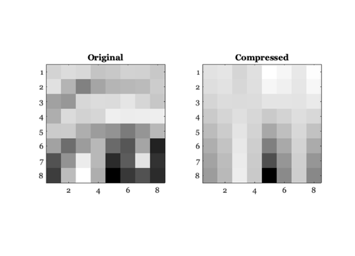
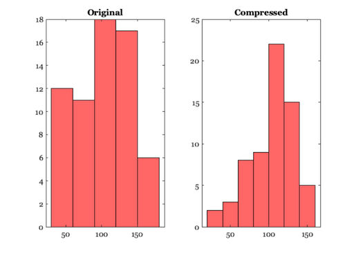
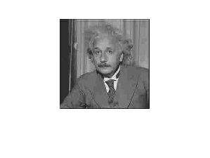
% Now we decode the stored quantized JPEG coefficients to get
% back an image.  To do this, we just need to invert the dct
% transformation. Again, we apply the decoding step to one 8x8
% block first to give you an idea of how it works.
%
block = im(89:96, 105:112);
blockdct = dctQuant(89:96, 105:112);
blockjpeg = idctMatrix*blockdct*idctMatrix';

% Here are the differences between the original and compressed
% block
round(blockjpeg) - block

% And here is a picture of the two blocks
vcNewGraphWin; colormap(linMap)
subplot(1,2,1); imagesc(block), axis image, title('Original')
subplot(1,2,2); imagesc(blockjpeg), axis image, title('Compressed')

% You can see that the reconstructed image intensities are spread
% out again, but not as spread out as the original.
vcNewGraphWin;
subplot(1,2,1); histogram(block(:)); title('Original')
subplot(1,2,2); histogram(blockjpeg(:)); title('Compressed')

% If we use the IDCT function in Matlab, the results should be
% the same:
% c = [ 1/sqrt(2) 1 1 1 1 1 1 1 ];
% blockjpeg1 = idct((blockdct*inv(diag(c))*8)');
% blockjpegm = idct((blockjpeg1*inv(diag(c))*8)');
% max(abs(blockjpegm(:) - blockjpeg(:)))

% Now we decode the whole image.
%
imjpeg = zeros(size(im));
for i=1:8:size(im,1)
    for j=1:8:size(im,2)
        block = dctQuant(i:i+7, j:j+7);
        imjpeg(i:i+7, j:j+7) = idctMatrix*block*idctMatrix';
    end
end

% The result of inverse DCT transform is not guarranteed to be
% within the [0 255] range, so we truncate it.
imjpeg = round(truncate(imjpeg, 0, 255));

% Now, let's see how well we did.
vcNewGraphWin;
imshow(imjpeg, gray(256));

% We can repeat this whole set of operations using this function
% we wrote, jpegCompress, but with a quality factor that makes
% the artifacts very visible.

vcNewGraphWin;
Q_factor = 30;
q1 = jpeg_qtables(Q_factor,1)
imjpeg2 = jpegCompress(im, q1);
imjpeg2 = truncate(imjpeg2, 0, 255);
imshow(imjpeg2, gray(256));
ans =

    -4    -9   -21     7    36    17     3    34
   -21    22    42    28    41    33    19    23
    23    35   -15   -19    -9   -19    -6    15
     3   -24    -6   -16   -53   -42   -34   -40
   -31   -19    27    23    -5    24    33   -10
   -10    34    44     0   -10    22    18    33
    19     9   -19    -3   -12     8   -36    18
    20   -22   -37     3   -19    10    52    11


q1 =

    27    18    20    23    20    17    27    23
    22    23    30    28    27    32    40    67
    43    40    37    37    40    82    58    62
    48    67    97    85   102   100    95    85
    93    92   107   120   153   130   107   113
   145   115    92    93   133   182   135   145
   158   163   172   173   172   103   128   188
   202   187   167   200   153   168   172   165
BEGIN TUTORIAL QUESTIONS
% Question 1: JPEG COMPRESSION OF GRAYSCALE IMAGE
%
% a) Describe the initial steps (the steps prior to quantization) in the
% JPEG-DCT computation in terms of convolution followed by sampling.
%
% b) At what point is information lost in the JPEG-DCT computation?
%
% c) Why is it better to quantize the JPEG-DCT coefficients rather than
% the intensities of individual pixels?
%
% d) Suppose you use a JPEG-DCT compressor to compress an image
% (yielding image a); then you uncompress the image and compress it
% again using the same compressor and compression settings (yielding
% image b). How will the two compressed images (a and b) compare?  Explain.
%
% e) What are the main visual artifacts present in JPEG-DCT compressed
% grayscale image?  What types of images will display artifacting most
% visibly?
%
% Question 2:
%
% Read the einstein.mat image, and compress it using JPEG quantization
% levels of 75, 50, 25, and 0.  You may want to use the imread and imwrite
% functions to accomplish this.  Normalize all images to have intensities
% from 0 to 1 (as opposed to 0 to 255).
%
% a) Submit the squared-error image for q=25.
%
% b) Describe where the error image has the highest values.  Does this
% agree with your understanding of the JPEG-DCT algorithm?
%
% c) For each compressed image, compute the mean squared error and plot the
% error vs. quantization factor. [You may obtain data for more quantization
% settings if you like, but this is not required.]
%
% d) For each error image, compute the 95th percentile error point.  If
% your error image is called errorim, you can find this value as follows:
%
%    serr = sort(errorim(:)); % sort the error values
%    error95 = serr( floor(0.95 * length(serr)) ); % get the 95th percentile
%
% Also plot error vs quantization factor for this method.
%
% e) If you were evaluating image quality for this image, which method
% (c) or (d) would you use?  Describe why you would use this method.