Illustrate how to control of the image processing routines

Illuminant correction and demosaicking are illustrated.

Copyright ImagEval Consultants, LLC, 2007.

Contents

ieInit

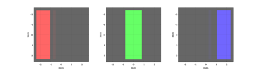
First, create a simple colorful test scene

scene  = sceneCreate('macbeth tungsten');
oi     = oiCreate;
sensor = sensorCreate;
sensor = sensorSet(sensor,'size',[340 420]);

% Match the scene field of view to the sensor size
fov = sensorGet(sensor,'fov',sceneGet(scene,'distance'),oi);
scene  = sceneSet(scene,'fov',fov);

% Compute the optical image and sensor from the scene.
oi     = oiCompute(oi,scene);
sensor = sensorCompute(sensor,oi);
ieAddObject(sensor);

We are ready to create and experiment with the image processing calls.

% Create the image processor.
ip = ipCreate;
ip = ipSet(ip,'name','default');

% First, we compute using the default image processing pipeline.
% Reading the boxes on the right of the window, we see the default
% processing steps.  These are
%
%  * Bilinear demosaicking
%  * Converting the sensor data into a calibrated internal color space
%  * Correcting for the illumination
%
% The demosaicking algorithm is implemented in Demosaic.m
% The sensor conversion in the default uses this logic:
%   * We know the sensor spectral responsivities
%   * We find the 3x3 linear transformation that best maps (least-squares)
%     the sensor values into a calibrated color space (See notes below).
%

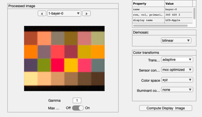
Set the sensor correction parameters

% Choose the internal color space
ip = ipSet(ip,'internal cs','XYZ');

% Choose the likely set of signals the sensor will encounter
ip = ipSet(ip,'conversion method sensor','MCC Optimized');

% Give the image processor a name
ip = ipSet(ip,'name','MCC-XYZ');

% Note that at this point we have left illuminant correction to 'None'.  So
% there will be no illuminant correction at this point.

% Compute from sensor to sRGB
ip = ipCompute(ip,sensor);
ipWindow(ip);

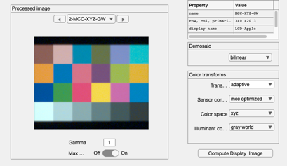
Set the illuminant correction algorithm

% We have only three default options at this point.
ip = ipSet(ip,'illuminant correction method','gray world');
ip = ipCompute(ip,sensor);
ip = ipSet(ip,'name','MCC-XYZ-GW');
ieAddObject(ip);
ipWindow;

Now, illustrate a different demosaic algorithm

ip = ipSet(ip,'demosaic method','Adaptive Laplacian');
ip = ipCompute(ip,sensor);
ip = ipSet(ip,'name','MCC-XYZ-GW-AL');
ieAddObject(ip);
ipWindow;

How the sensor conversion matrix is calculated

The transformation is calculated by predicting the sensor responses to a
MCC under D65 and then finding the 3x3 matrix that maps the sensor
values into the correct MCC values for a D65 light

Interacting with the image processing display

% This is the display structure
d = ipGet(ip,'display');
disp(d)

% There is a separate window for interacting with the display
% See t_displayIntroduction.

          type: 'display'
          name: 'LCD-Apple'
          wave: [31×1 double]
           spd: [31×3 double]
         gamma: [1024×3 double]
           dpi: 96
          dist: 0.5000
    isEmissive: 1
         dixel: [1×1 struct]
       ambient: [31×1 double]
         image: []

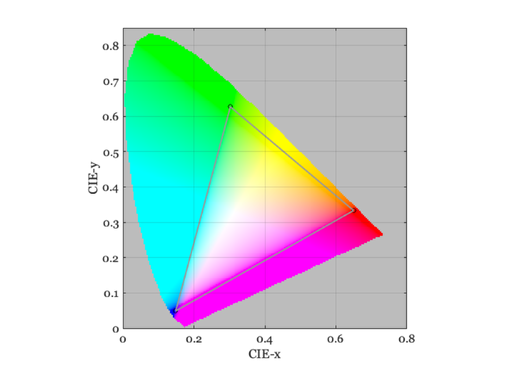
This is an image the display gamut in chromaticity coordinates

displayPlot(d,'gamut');

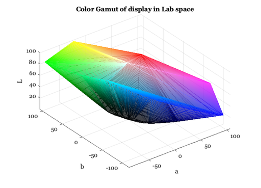
The display volume in Lab space

displayPlot(d,'gamut 3d');

Display subpixel pointspreads

displayPlot(d,'psf')

END

Published with MATLAB® R2024a