Calculate sensor conversion matrices for a surface reflectance chart.

Sensor conversion is a transformation, often implemented by a matrix multiply, that transforms the sensor data into a calibrated color space. An example is the CIE-XYZ space.

In this script we examine the stability of the best transformation matrix under different illuminants.

Several of the analyses are performed using the calibrated Nikon camera sensor spectral responsivities.

Copyright ImagEval Consultants, LLC, 2010

Contents

ieInit;

Choose scene surface reflectances

% Choose reflectance data for testing
sFiles = cell(1,2);
sFiles{1} = which('MunsellSamples_Vhrel.mat');
sFiles{2} = which('Food_Vhrel.mat');

%{
sFiles{1} = fullfile(isetRootPath,'data','surfaces','reflectances','MunsellSamples_Vhrel.mat');
sFiles{2} = fullfile(isetRootPath,'data','surfaces','reflectances','Food_Vhrel.mat');
%}
% Number of samples from each of the files
sSamples = [48 16];
% pSize = 16; [scene, samples] = sceneReflectanceChart(sFiles,sSamples,pSize);
% sceneWindow(scene);

Choose illuminant blackbodies

bbodyList = (3000:1000:8500);
nIlluminant = length(bbodyList);

% For plotting CIELAB dE graphs on a common scale
maxDE = 8;

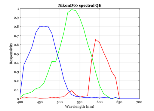
Create a Nikon sensor with an infrared cut filter.

% Load up  Nikon color filters and an infrared
nikon = sensorCreate;
wave  = sensorGet(nikon,'wave');
nikon = sensorSet(nikon,'infrared',ieReadSpectra('infrared2',wave));
filterFile = 'NikonD70';
nikon = sensorSet(nikon,'color filters',ieReadSpectra(filterFile,wave));

% Plot the Nikon spectral QE.
sqe = sensorGet(nikon,'spectral qe');

ieNewGraphWin;
p = plot(wave,sqe(:,1),'r-',wave,sqe(:,2),'g-',wave,sqe(:,3),'b-');
set(p,'linewidth',2); grid on
xlabel('Wavelength (nm)'); ylabel('Responsivity');
title(sprintf('%s spectral QE',filterFile));

Estimated sensor correction transforms for the different illuminants

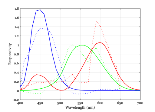
reflectances = ieReflectanceSamples(sFiles,sSamples);
T       = cell(1,nIlluminant);
actual  = cell(1,nIlluminant);
desired = cell(1,nIlluminant);
CMF = ieReadSpectra('XYZ.mat',wave);

% imageSensorConversion returns the transform, T, that converts the sensor
% data to the desired CMF representation.
for ii = 1:nIlluminant
    illuminant = blackbody(wave,bbodyList(ii));
    [T{ii}, actual{ii}, desired{ii}, whiteCMF] = ...
        imageSensorConversion(nikon,CMF,reflectances,illuminant);
end

% In this case, the T{ii} matrices convert the Nikon spectral QE to
% something close to the XYZ.
estXYZ = (T{3}*sqe')';

% Let's plot the transformed spectral QE for the 5000K illuminant
ieNewGraphWin;
p = plot(wave,estXYZ(:,1),'r:',wave,estXYZ(:,2),'g:',wave,estXYZ(:,3),'b:',...
    wave,CMF(:,1),'r-',wave,CMF(:,2),'g-',wave,CMF(:,3),'b');
set(p,'linewidth',2);
xlabel('Wavelength (nm)');
ylabel('Responsivity');
hold off; grid on

Not correctly implemented

scene = sceneCreate;
oi    = oiCreate;
oi    = oiCompute(oi,scene);
nikon = sensorSet(nikon,'fov',sceneGet(scene,'fov'),oi);
nikon = sensorCompute(nikon,oi);
sensorWindow(nikon);

Plot the corrected and desired for each illuminant case

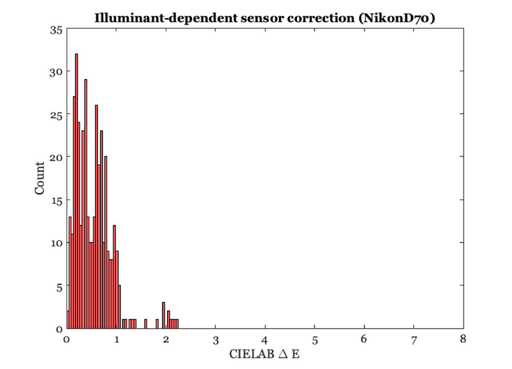
% Store the CIELAB delta E here
dE = cell(1,nIlluminant);

% T(3x3)*sensorData(3xN) is supposed to be XYZ
for ii=1:nIlluminant
    corrected = T{ii}*actual{ii};
    dE{ii} = deltaEab(corrected',desired{ii}',whiteCMF);
end

allDE = [];
for ii=1:nIlluminant
    allDE = [allDE, dE{ii}]; %#ok<AGROW>
end

ieNewGraphWin;
histogram(allDE,50);
set(gca,'xlim',[0 maxDE])
xlabel('CIELAB \Delta E'); ylabel('Count')
title(sprintf('Illuminant-dependent sensor correction (%s)',filterFile));

% close all

Use the average of the linear transformations

tmp = zeros(size(T{1}));
for ii=1:nIlluminant, tmp = tmp + T{ii}; end
Tave = tmp/nIlluminant;

for ii=1:nIlluminant
    corrected = Tave*actual{ii};
    dE{ii} = deltaEab(corrected',desired{ii}',whiteCMF);
end

allDE = [];
for ii=1:nIlluminant
    allDE = [allDE, dE{ii}]; %#ok<AGROW>
end

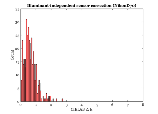
ieNewGraphWin;
histogram(allDE,50);
set(gca,'xlim',[0 maxDE])
xlabel('CIELAB \Delta E')
ylabel('Count')
title(sprintf('Illuminant-independent sensor correction (%s)',filterFile));

fprintf('%s',filterFile)
Tave %#ok<NOPTS>
s = svd(Tave);
fprintf('Condition number: %f\n',s(1)/s(3));

NikonD70
Tave =

    2.2475    0.1414    0.1793
    1.0149    0.9329   -0.2429
    0.0176   -0.1268    1.7180

Condition number: 3.455386

Create a sensor with different filters. (CYM)

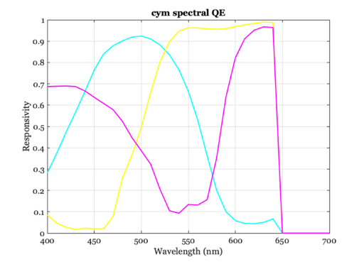
% Set the sensor of interest here
sensor = sensorCreate;
wave   = sensorGet(sensor,'wave');

% Load up CYM color filters
sensor = sensorSet(sensor,'infrared',ieReadSpectra('infrared2',wave));
filterFile = 'cym';
sensor = sensorSet(sensor,'color filters',ieReadSpectra(filterFile,wave));
sensor = sensorSet(sensor,'name','CMY');
sqe    = sensorGet(sensor,'spectral qe');

ieNewGraphWin;
p = plot(wave,sqe(:,1),'c-',wave,sqe(:,2),'y-',wave,sqe(:,3),'m-');
set(p,'linewidth',2); grid on
xlabel('Wavelength (nm)'); ylabel('Responsivity')
title(sprintf('%s spectral QE',filterFile));

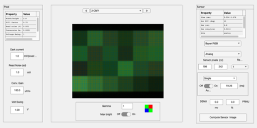
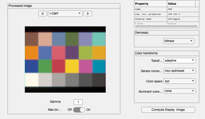
scene = sceneCreate;
oi    = oiCreate;
oi    = oiCompute(oi,scene);
sensor = sensorSet(sensor,'fov',sceneGet(scene,'fov'),oi);
sensor = sensorCompute(sensor,oi);
sensorWindow(sensor);

ip = ipCreate;
ip = ipCompute(ip,sensor);
ipWindow(ip);

Estimated sensor correction transforms for the different illuminants

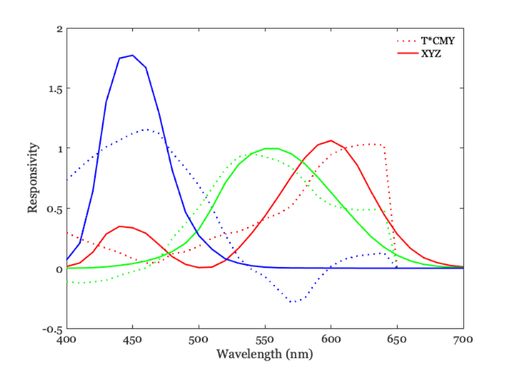
reflectances = ieReflectanceSamples(sFiles,sSamples);
T       = cell(1,nIlluminant);
actual  = cell(1,nIlluminant);
desired = cell(1,nIlluminant);
CMF = ieReadSpectra('XYZ.mat',wave);

for ii = 1:nIlluminant
    illuminant = blackbody(wave,bbodyList(ii));
    [T{ii}, actual{ii}, desired{ii}, whiteCMF] = ...
        imageSensorConversion(sensor,CMF,reflectances,illuminant);
end

% The T{ii} matrices convert the Nikon spectral QE to something close to
% the XYZ.
estXYZ = (T{3}*sqe')';

% Let's plot these for the 5000K illuminant
ieNewGraphWin;
p = plot(wave,estXYZ(:,1),'r:',wave,estXYZ(:,2),'g:',wave,estXYZ(:,3),'b:',...
    wave,CMF(:,1),'r-',wave,CMF(:,2),'g-',wave,CMF(:,3),'b');
set(p,'linewidth',2)
xlabel('Wavelength (nm)'); ylabel('Responsivity');
l = legend(p([1,4]),{'T*CMY','XYZ'}); set(l,'Box','off','Color','none')
hold off

Plot the corrected and desired for each illuminant case

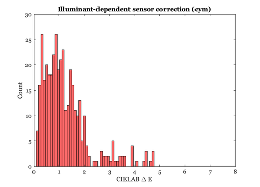
% These are really pretty good for the Nikon spectral QE
dE = cell(1,nIlluminant);
for ii=1:nIlluminant
    corrected = T{ii}*actual{ii};
    dE{ii} = deltaEab(corrected',desired{ii}',whiteCMF);
end

allDE = [];
for ii=1:nIlluminant
    allDE = [allDE, dE{ii}]; %#ok<AGROW>
end

% Error in CIELAB space
ieNewGraphWin;
histogram(allDE,50);
set(gca,'xlim',[0 maxDE])
xlabel('CIELAB \Delta E'); ylabel('Count')
title(sprintf('Illuminant-dependent sensor correction (%s)',filterFile));

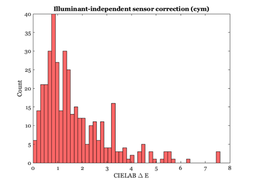
Use the average of the linear transformations to compute delta E

tmp = zeros(size(T{1}));
for ii=1:nIlluminant, tmp = tmp + T{ii}; end
Tave = tmp/nIlluminant;

for ii=1:nIlluminant
    corrected = Tave*actual{ii};
    dE{ii} = deltaEab(corrected',desired{ii}',whiteCMF);
end

allDE = [];
for ii=1:nIlluminant
    allDE = [allDE, dE{ii}]; %#ok<AGROW>
end

ieNewGraphWin;
histogram(allDE,50);
set(gca,'xlim',[0 maxDE])
xlabel('CIELAB \Delta E')
ylabel('Count')
title(sprintf('Illuminant-independent sensor correction (%s)',filterFile));

% Tell the user about the condition number
fprintf('%s',filterFile)
Tave %#ok<NOPTS>
s = svd(Tave);
fprintf('Condition number: %f\n',s(1)/s(3));

cym
Tave =

   -0.3225    0.5846    0.4856
    0.2450    0.8471   -0.3738
    0.7889   -0.7251    0.8168

Condition number: 2.195921

Published with MATLAB® R2024a