Measure the modulation transfer function (MTF) of a test target

Use the Mackay pattern as an input. Then, select data from a series of circles of increasing radius. Measure the MTF as a function of radius.

See also: ipCompute, ipGet,

Copyright ImagEval Consultants, LLC, 2010

Contents

ieInit

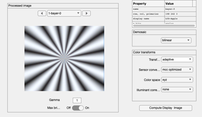
scene = sceneCreate('mackay');
oi    = oiCreate;
oi    = oiCompute(oi,scene);
sensor= sensorCreate;
sensor= sensorSet(sensor,'fov',sceneGet(scene,'fov'),oi);
sensor= sensorCompute(sensor,oi);

ip    = ipCreate;
ip    = ipCompute(ip,sensor);

ipWindow(ip);

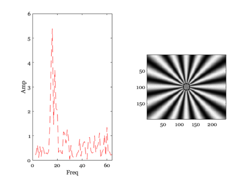
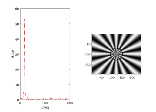
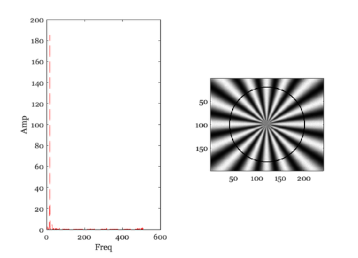
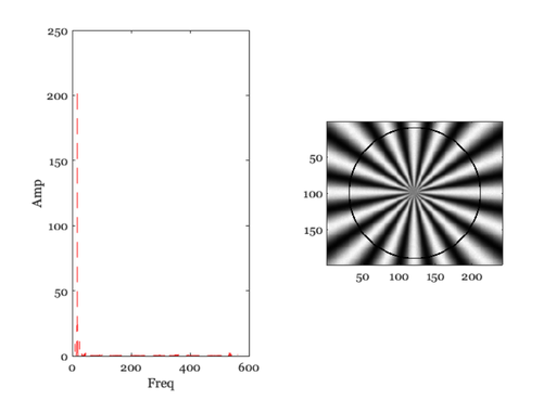
Plot spectrum and the circle on the data ...

% Get the distance to the center for each pixel
d2c = ipGet(ip,'distance 2 center');

% Get the angle of each pixel
ang = ipGet(ip,'angle');

% Get a list of radii for circles
rList = 10:10:(min(size(ang)/2)*0.95);

img = ipGet(ip,'result');
rImg = img(:,:,2);
% figure(1); imagesc(rImg); axis image
thisPeak = zeros(1,length(rList));

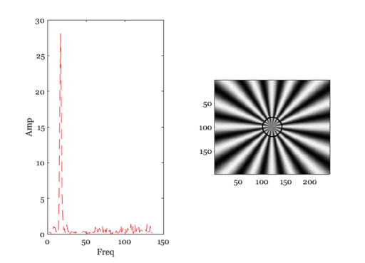
for ii=1:length(rList)
    ieNewGraphWin;
    tiledlayout(1,2);

    % Find the points at this distance
    lst = (abs(d2c - rList(ii)) < 1);  % figure; imagesc(l)
    [thisAng, ix]= sort(ang(lst));

    thisVal = rImg(lst);
    thisVal = thisVal(ix);

    % Compute the spectral power distribution
    spec = abs(fft(thisVal));

    % These are the number of points
    n = floor(length(spec)/2);

    % Save the peak above DC.  We should really save the frequency term
    % that we are interested in.  But that's too hard to find right now.
    % Do it later. I think it is just the number of cycles in the pattern.
    thisPeak(ii) = max(spec(2:n));

    nexttile; plot(2:n,spec(2:n),'--');
    xlabel('Freq'); ylabel('Amp');

    % Show the circle on the image
    nexttile; tmp = rImg; tmp(lst) = 0;
    imagesc(tmp); colormap(gray(256)); axis image; pause(2);
end

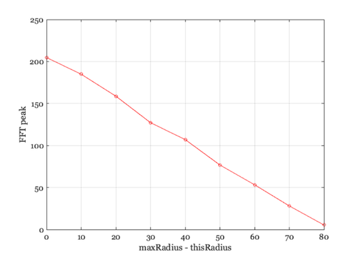
Plot the modulation transfer function

ieNewGraphWin;
plot(max(rList) - rList,thisPeak,'o-')
xlabel('maxRadius - thisRadius')
ylabel('FFT peak')
grid on

Published with MATLAB® R2024a