Introduction to ISETCam
An overview of ISETCam illustrating how to perform basic image system simulation.
To find through other example scripts and tutorials use the tab-completion function. For example
- Use t_"TAB KEY" to see the list of tutorials
- Use s_"TAB KEY" to see the list of ISET scripts
- Use s_scene"TAB KEY" to see the scripts related to scenes
To learn more about the processing for a particular function, type using Matlab's doc command, suhc as doc sceneCreate.
See also: t_sceneIntroduction.m and t_oiIntroduction.m
Copyright ImagEval Consultants, LLC, 2010.
Contents
- Initialize ISET variables and structures
- Scene spectral radiance
- The scene illuminant
- It is possible to change the scene illuminant
- Optics
- Calculate the optical image (irradiance at the sensor)
- Sensor
- Image Processor
- You can experiment by changing the processing parameters
- How to reduce the chromatic aliasing
- END
Initialize ISET variables and structures
The ieInit function closes windows and can clear your variables, depending on how you set your ISET preferences.
% Here is how your preferences are set
getpref('ISET')   % Current status

% To clear workspace variables on ieInit, do this
setpref('ISET','initclear',true);

% To preserve workspace variables on ieInit, do this
setpref('ISET','initclear',false);

ieInit;
ans =

  struct with fields:

                        initclear: 0
                          waitbar: 1
                        fontDelta: 8
                             wPos: {7×1 cell}
                         fontSize: 14
                 maxSearchResults: 20
                  openRGBwavelist: [400 410 420 430 440 450 … ] (1×31 double)
                    keepDownloads: 0
                   benchmarkstart: 2.7182e+04
    maxSharingSiteImageResolution: 512
                           wState: {[]  'normal'  'normal'  'normal'  'normal'}
                      customicons: 0
                           tStart: 369376814742920
                     tvsceneStart: 369376836180610
                        useSingle: 1
                      tvsceneTime: 45.2016
                    tvopticsStart: 369114618304515
                     tvopticsTime: 29.2217
                    tvsensorStart: 369143860666969
                     tvsensorTime: 25.4201
                     tvpixelStart: 369169301584421
                      tvpixelTime: 3.9278
                     tvhumanStart: 369173251195648
                      tvhumanTime: 14.1937
                        tvipStart: 369187467012507
                         tvipTime: 7.8952
                   tvmetricsStart: 369195384498678
                    tvmetricsTime: 35.5002
                   tvdisplayStart: 369230972961491
                    tvdisplayTime: 6.6743
                         fastAxes: 0
                  fast_num2string: 0
                        tvciStart: 369230907627415
                         tvciTime: 0.0434
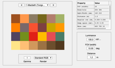
Scene spectral radiance
There are several ways to create a scene. One is to use the sceneCreate function. In the example below, we create a scene of the Macbeth Color Checker illuminated with a tungsten light For a complete list of the types of synthetic scenes type doc sceneCreate.
A second method for creating a scene is to read data from a file. ISET includes a few multispectral scenes as part of the distribution. These can be found in the data/image/multispectral directory You can also select the file (or many other files) using the command:
* fullFileName = vcSelectImage;*
See also: s_sceneFromMultispectral.m, s_sceneFromRGB.m and scripts/scenes
wave = 400:10:700;
patchSize = 64;
scene = sceneCreate('macbeth tungsten',patchSize,wave);

% It is often useful to visualize the data in the scene window
sceneWindow(scene);
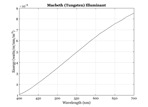
The scene illuminant
Within the ISET framework, we use specific functions to interact with the objects. All of the major types of objects have a Create, Get, Set and Plot function. For example, to plot the illuminant of a scene, you can use scenePlot();
scenePlot(scene,'illuminant energy roi');
No ROI needed unless spatial spectral illluminant
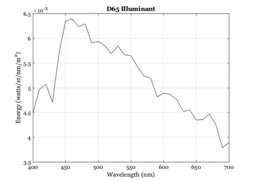
It is possible to change the scene illuminant
There are also many different utilities that do useful things. For example to change the illuminant spectral power distribution use this code.
scene = sceneAdjustIlluminant(scene,'D65.mat');
scene = sceneSet(scene,'name','D65'); % Set the scene name
scenePlot(scene,'illuminant energy roi');
No ROI needed unless spatial spectral illluminant
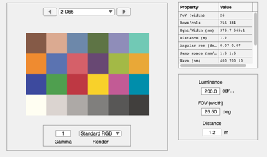
You can adjust properties using the sceneSet command. Here we adjust the scene mean luminance and field of view.
scene = sceneAdjustLuminance(scene,200);  % Candelas/m2
scene = sceneSet(scene,'fov',26.5);       % Set the scene horizontal field of view
scene = sceneInterpolateW(scene,wave,true); % Resample, preserve luminance
sceneWindow(scene);            % if you want to view the change in the GUI window
Optics
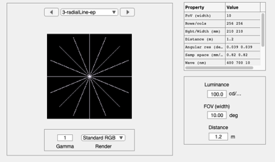
There are also simple functions to transform between the objects, say from the scene (radiance) to the optical image (irradiance). To explore the effect of optics let's use a scene with lots of radial lines. This is one of the many 'baked' test images. You can see all of them and how to adjust their parameters by typing doc sceneCreate.
scene = sceneCreate('radial lines');
sceneWindow(scene);
Calculate the optical image (irradiance at the sensor)
The optical image is an important structure, like the scene structure. We adjust the properties of optical image formation using the oiSet and oiGet routines.
ISET has several optics models that you can experiment with. These include shift-invariant optics, in which there is a different shift-invariant pointspread function for each wavelength, and a ray-trace method, in which we read in data from Zemax and create a shift-variant set of pointspread functions along with a geometric distortion function.
oi = oiCreate;

% The simplest is method of creating an optical image is to use
% the diffraction-limited lens model.  To create diffraction
% limited optics with an f# of 12, which will blur the image substantially,
% you can call these functions
oi = oiSet(oi,'optics fnumber',2.8);

% In this example we set the properties of the optics to include
% cos4th falloff for the off axis vignetting of the imaging lens
% and we set the lens focal length to 3 mm.
oi = oiSet(oi,'optics offaxis method','cos4th');
oi = oiSet(oi,'optics focal length',3e-3);
oi = oiCompute(oi,scene);

% Save the optical image structure and bring up the optical image
% window.
oiWindow(oi);
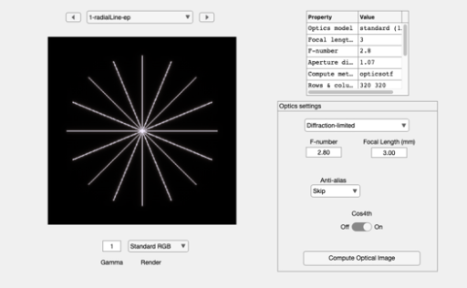
Many other optics and oi properties can be set . For a list see doc opticsSet, and doc oiSet.
We use the scene structure and the optical image structure to update the irradiance. From the window you can see a wide range of options. These include insertion of a birefringent anti-aliasing filter, turning off cos4th image fall-off, adjusting the lens properties, and so forth.
You can read more about optics models properties by typing doc opticsGet.
Sensor
% The irradiance is then captured by a simulated sensor,
% resulting in an array of output voltages. There are a very
% large number of sensor parameters. Here we illustrate the
% process of creating a simple Bayer-gbrg sensor and setting a
% few of its basic properties.
%
% To create the sensor structure, we call
sensor = sensorCreate('bayer (rggb)');

% We set the sensor properties using *sensorSet* and *sensorGet*
% routines.
%
% Just as the optical irradiance gives a special status to the
% optics, the sensor gives a special status to the pixel.  In
% this section we define the key pixel and sensor properties, and
% we then put the sensor and pixel back together.

% To get the pixel structure from the sensor we use:
pixel =  sensorGet(sensor,'pixel');

% Here are some of the key pixel properties
voltageSwing   = 1.15;  % Volts
wellCapacity   = 9000;  % Electrons
conversiongain = voltageSwing/wellCapacity;
fillfactor     = 0.45;       % A fraction of the pixel area
pixelSize      = 2.2*1e-6;   % Meters
darkvoltage    = 1e-005;     % Volts/sec
readnoise      = 0.00096;    % Volts

% We set the pixel properties here.
sensor = sensorSet(sensor,'pixel size same fill factor',[pixelSize pixelSize]);
sensor = sensorSet(sensor,'pixel conversion gain', conversiongain);
sensor = sensorSet(sensor,'pixel voltage swing',voltageSwing);
sensor = sensorSet(sensor,'pixel dark voltage',darkvoltage) ;
sensor = sensorSet(sensor,'pixel read noise volts',readnoise);

%  Now we set some general sensor properties
dsnu =  0.0010;           % Volts (dark signal non-uniformity)
prnu = 0.2218;            % Percent (ranging between 0 and 100) photodetector response non-uniformity
analogGain   = 1;         % Used to adjust ISO speed
analogOffset = 0;         % Used to account for sensor black level
rows = 466;               % number of pixels in a row
cols = 642;               % number of pixels in a column

% Set sensor properties
sensor = sensorSet(sensor,'auto exposure',true);
% N.B. You could set the exposure duration explicitly using
% sensor = sensorSet(sensor,'exp time',0.030);

% Some other
sensor = sensorSet(sensor,'rows',rows);
sensor = sensorSet(sensor,'cols',cols);
sensor = sensorSet(sensor,'dsnu level',dsnu);
sensor = sensorSet(sensor,'prnu level',prnu);
sensor = sensorSet(sensor,'analog Gain',analogGain);
sensor = sensorSet(sensor,'analog Offset',analogOffset);

% Adjust the pixel fill factor
sensor = pixelCenterFillPD(sensor,fillfactor);

% It is also possible to replace the spectral quantum efficiency curves of
% the sensor with those from a calibrated camera.  We include the
% calibration data from a very nice Nikon D100 camera as part of ISET.
% To load those data we first determine the wavelength samples for this sensor.
wave = sensorGet(sensor,'wave');

% Then we load the calibration data and attach them to the sensor structure
fullFileName = fullfile(isetRootPath,'data','sensor','colorfilters','nikon','NikonD100.mat');
[data,filterNames] = ieReadColorFilter(wave,fullFileName);
sensor = sensorSet(sensor,'filter spectra',data);
sensor = sensorSet(sensor,'filter names',filterNames);
sensor = sensorSet(sensor,'Name','Camera-Simulation');

% We are now ready to compute the sensor image
sensor = sensorCompute(sensor,oi);

% We can view sensor image in the GUI.  Note that the image that
% comes up shows the color of each pixel in the sensor mosaic.
% Also, please be aware that the Matlab rendering algorithm often
% introduces unwanted artifacts into the display window.  You can
% resize the window to eliminate these. You can also set the
% display gamma function to brighten the appearance in the edit
% box at the lower left of the window.
sensorWindow(sensor);

% There are a variety of ways to quantify these data in the
% pulldown menus. Also, you can view the individual pixel data
% either by zooming on the image (Edit | Zoom) or by bringing the
% image viewer tool (Edit | Viewer).
%
% See also: *iexL2ColorFilter*
%
% ISET includes a wide array of options for selecting color
% filters, fill-factors, infrared blocking filters, adjusting
% pixel properties, color filter array patterns, and exposure
% modes.
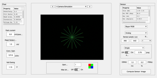
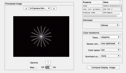
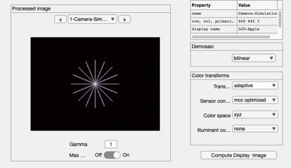
Image Processor
The sensor array is demosaiced, color-balanced, and rendered on a display The image processing pipeline is managed by the fourth principal ISET structure, the virtual camera image (ip). This structure allows the user to set a variety of image processing methods, including demosaicking and color balancing.
ip = ipCreate;

% The routines for setting and getting image processing
% parameters are ipGet and ipSet.
%
ip = ipSet(ip,'name','Unbalanced');
ip = ipSet(ip,'scale display',1);

% The default properties use bilinear demosaicking, no color
% conversion or balancing.  The sensor RGB values are simply set
% to the display RGB values.
ip = ipCompute(ip,sensor);

% As in the other cases, we can bring up a window to view the
% processed data, this time a full RGB image.
ieAddObject(ip); ipWindow
ans =

  ipWindow_App with properties:

                        figure1: [1×1 Figure]
                       menuFile: [1×1 Menu]
                   menuFileLoad: [1×1 Menu]
           menuFileSaveProcData: [1×1 Menu]
              menuFileLoadImage: [1×1 Menu]
                   menuFileSave: [1×1 Menu]
                menuFileRefresh: [1×1 Menu]
                  menuFileClose: [1×1 Menu]
                       menuEdit: [1×1 Menu]
                   menuEditName: [1×1 Menu]
                 menuEditCreate: [1×1 Menu]
              menuEditCopyImage: [1×1 Menu]
                 menuEditDelete: [1×1 Menu]
             menuEditDeleteSome: [1×1 Menu]
                 menuImageWhite: [1×1 Menu]
             menuEditResetWhite: [1×1 Menu]
             menuScaleChooseMax: [1×1 Menu]
               menuScaleDisplay: [1×1 Menu]
               menuEditFontSize: [1×1 Menu]
           menuEditClearMessage: [1×1 Menu]
                 menuEditViewer: [1×1 Menu]
                       menuPlot: [1×1 Menu]
               menuPlImTrueSize: [1×1 Menu]
               multipleImageRGB: [1×1 Menu]
                menuPlotDisplay: [1×1 Menu]
                 plotDisplaySPD: [1×1 Menu]
                      plotGamut: [1×1 Menu]
    plotColorProcessingMatrices: [1×1 Menu]
                 plotMCCOverOff: [1×1 Menu]
                    menuDisplay: [1×1 Menu]
                    menuReadSPD: [1×1 Menu]
              menuDisplayWindow: [1×1 Menu]
               menuDisplayViewD: [1×1 Menu]
                    menuAnalyze: [1×1 Menu]
                    menuAnColor: [1×1 Menu]
                      menuAnROI: [1×1 Menu]
                      menuAnLum: [1×1 Menu]
                    menuAnChrom: [1×1 Menu]
                 menuAnColorLAB: [1×1 Menu]
                      menuAnLUV: [1×1 Menu]
                    menuRGBHist: [1×1 Menu]
                  menuAnROIvSNR: [1×1 Menu]
          chartClearcornersMenu: [1×1 Menu]
                        MCCMenu: [1×1 Menu]
             LuminancenoiseMenu: [1×1 Menu]
           ColormetricssRGBMenu: [1×1 Menu]
           VisualcompareD65Menu: [1×1 Menu]
                     menuAnLine: [1×1 Menu]
                    menuAnLineH: [1×1 Menu]
                    menuAnLineV: [1×1 Menu]
            menuAnalyzeCreateSB: [1×1 Menu]
            menuAnalyzeISO12233: [1×1 Menu]
              menuMetricsWindow: [1×1 Menu]
        menuAnComputeFromSensor: [1×1 Menu]
              menuComputeFromOI: [1×1 Menu]
         menuAnComputeFromScene: [1×1 Menu]
                       menuHelp: [1×1 Menu]
        menuHelpProcessorOnline: [1×1 Menu]
              menuHelpMetricsPG: [1×1 Menu]
             menuHelpISETOnline: [1×1 Menu]
               menuHelpAppNotes: [1×1 Menu]
                     btnCompute: [1×1 Button]
                  DemosaicPanel: [1×1 Panel]
                    popDemosaic: [1×1 DropDown]
           ColortransformsPanel: [1×1 Panel]
                      txtSensor: [1×1 Label]
                  txtIlluminant: [1×1 Label]
                     popBalance: [1×1 DropDown]
                         txtICS: [1×1 Label]
                  popColorSpace: [1×1 DropDown]
                      txtMethod: [1×1 Label]
            popColorConversionM: [1×1 DropDown]
                   popTransform: [1×1 DropDown]
                        ipTable: [1×1 Table]
            ProcessedimagePanel: [1×1 Panel]
                MaxbrightSwitch: [1×1 Switch]
           MaxbrightSwitchLabel: [1×1 Label]
                     txtMessage: [1×1 Label]
                      editGamma: [1×1 EditField]
                         text10: [1×1 Label]
                        btnPrev: [1×1 Button]
                        btnNext: [1×1 Button]
                      popSelect: [1×1 DropDown]
                        ipImage: [1×1 UIAxes]
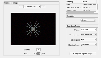
You can experiment by changing the processing parameters
% For example
ip2 = ipSet(ip,'name','More Balanced');
ip2 = ipSet(ip2,'internalCS','XYZ');
ip2 = ipSet(ip2,'conversion method sensor','MCC Optimized');
ip2 = ipSet(ip2,'correction method illuminant','Gray World');

% With these parameters, the colors will appear to be more accurate
ip2 = ipCompute(ip2,sensor);

ipWindow(ip2)

% Again, this window offers the opportunity to perform many
% parameter changes and to evaluate certain metric properties of
% the current system. Try the pulldown menu item (Analyze |
% Create Slanted Bar) and then run the pulldown menu (Analyze |
% ISO12233) to obtain a spatial frequency response function for
% the slanted bar image in the ISO standard.
ans =

  ipWindow_App with properties:

                        figure1: [1×1 Figure]
                       menuFile: [1×1 Menu]
                   menuFileLoad: [1×1 Menu]
           menuFileSaveProcData: [1×1 Menu]
              menuFileLoadImage: [1×1 Menu]
                   menuFileSave: [1×1 Menu]
                menuFileRefresh: [1×1 Menu]
                  menuFileClose: [1×1 Menu]
                       menuEdit: [1×1 Menu]
                   menuEditName: [1×1 Menu]
                 menuEditCreate: [1×1 Menu]
              menuEditCopyImage: [1×1 Menu]
                 menuEditDelete: [1×1 Menu]
             menuEditDeleteSome: [1×1 Menu]
                 menuImageWhite: [1×1 Menu]
             menuEditResetWhite: [1×1 Menu]
             menuScaleChooseMax: [1×1 Menu]
               menuScaleDisplay: [1×1 Menu]
               menuEditFontSize: [1×1 Menu]
           menuEditClearMessage: [1×1 Menu]
                 menuEditViewer: [1×1 Menu]
                       menuPlot: [1×1 Menu]
               menuPlImTrueSize: [1×1 Menu]
               multipleImageRGB: [1×1 Menu]
                menuPlotDisplay: [1×1 Menu]
                 plotDisplaySPD: [1×1 Menu]
                      plotGamut: [1×1 Menu]
    plotColorProcessingMatrices: [1×1 Menu]
                 plotMCCOverOff: [1×1 Menu]
                    menuDisplay: [1×1 Menu]
                    menuReadSPD: [1×1 Menu]
              menuDisplayWindow: [1×1 Menu]
               menuDisplayViewD: [1×1 Menu]
                    menuAnalyze: [1×1 Menu]
                    menuAnColor: [1×1 Menu]
                      menuAnROI: [1×1 Menu]
                      menuAnLum: [1×1 Menu]
                    menuAnChrom: [1×1 Menu]
                 menuAnColorLAB: [1×1 Menu]
                      menuAnLUV: [1×1 Menu]
                    menuRGBHist: [1×1 Menu]
                  menuAnROIvSNR: [1×1 Menu]
          chartClearcornersMenu: [1×1 Menu]
                        MCCMenu: [1×1 Menu]
             LuminancenoiseMenu: [1×1 Menu]
           ColormetricssRGBMenu: [1×1 Menu]
           VisualcompareD65Menu: [1×1 Menu]
                     menuAnLine: [1×1 Menu]
                    menuAnLineH: [1×1 Menu]
                    menuAnLineV: [1×1 Menu]
            menuAnalyzeCreateSB: [1×1 Menu]
            menuAnalyzeISO12233: [1×1 Menu]
              menuMetricsWindow: [1×1 Menu]
        menuAnComputeFromSensor: [1×1 Menu]
              menuComputeFromOI: [1×1 Menu]
         menuAnComputeFromScene: [1×1 Menu]
                       menuHelp: [1×1 Menu]
        menuHelpProcessorOnline: [1×1 Menu]
              menuHelpMetricsPG: [1×1 Menu]
             menuHelpISETOnline: [1×1 Menu]
               menuHelpAppNotes: [1×1 Menu]
                     btnCompute: [1×1 Button]
                  DemosaicPanel: [1×1 Panel]
                    popDemosaic: [1×1 DropDown]
           ColortransformsPanel: [1×1 Panel]
                      txtSensor: [1×1 Label]
                  txtIlluminant: [1×1 Label]
                     popBalance: [1×1 DropDown]
                         txtICS: [1×1 Label]
                  popColorSpace: [1×1 DropDown]
                      txtMethod: [1×1 Label]
            popColorConversionM: [1×1 DropDown]
                   popTransform: [1×1 DropDown]
                        ipTable: [1×1 Table]
            ProcessedimagePanel: [1×1 Panel]
                MaxbrightSwitch: [1×1 Switch]
           MaxbrightSwitchLabel: [1×1 Label]
                     txtMessage: [1×1 Label]
                      editGamma: [1×1 EditField]
                         text10: [1×1 Label]
                        btnPrev: [1×1 Button]
                        btnNext: [1×1 Button]
                      popSelect: [1×1 DropDown]
                        ipImage: [1×1 UIAxes]
How to reduce the chromatic aliasing
Increase the optical blur
oi = oiSet(oi,'optics fnumber',8);
oi = oiCompute(oi,scene);
sensor = sensorCompute(sensor,oi);
ip = ipCompute(ip,sensor);
ipWindow(ip);