Use color principles to create a spectrum (Psych 221)

Use the principles of color matching to render an approximation to the visible spectrum on a display.

Class: Psych 221/EE 362 Tutorial: Spectrum Author: Wandell Purpose: An example calculation: making a desaturated rainbow. Date: 01.12.98 Duration: 20 minutes

PURPOSE: This tutorial uses the color-matching tools to create an image approaching the appearance the rainbow (the spectral colors) on your display.

Contents

ieInit

Load the color matching functions

% These are are essential for creating calibrated signals.  So, we load
% them first.
wavelength = 390:730;
XYZ = ieReadSpectra('XYZ.mat',wavelength);

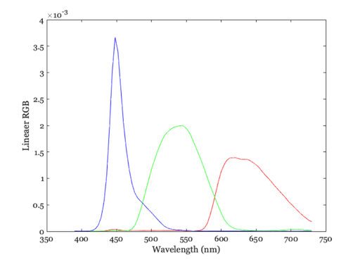
Model a display

% Let's suppose the spectral power distributions of your monitor's
% phosphors are from the LCD-APple.
d = displayCreate('LCD-Apple','wave',wavelength);
phosphors = displayGet(d,'spd');

% Here is a plot of the phosphors
vcNewGraphWin;
plot(wavelength,phosphors(:,1),'r', ...
    wavelength,phosphors(:,2),'g', ...
    wavelength,phosphors(:,3),'b')
xlabel('Wavelength(nm)'); ylabel('Energy (watts/st/m^2/nm');
set(gca,'xlim',[350 750]);
xlabel('Wavelength (nm)'); ylabel('Lineaer RGB');

Compute the conversion matrix

% This matrix converts between XYZ values and linear intensities of the
% monitor RGB values.

% We do this in two steps.  First, we find the XYZ values for each of the
% individual phosphors.  The columns of this matrix represent the XYZ
% values of the red, green and blue phosphors, respectively.  These values
% should be relatively easy to interpret.
%

rgb2xyz = XYZ'*phosphors

% Invert the rgb2xyz matrix so that we can compute from
% XYZ back to linear RGB values.
%

xyz2rgb = inv(rgb2xyz)

% Notice that the values of the xyz2rgb matrix contain negative
% values and are difficult to interpret directly. Such is life.

rgb2xyz =

    0.0673    0.0622    0.0297
    0.0345    0.1287    0.0097
    0.0017    0.0146    0.1608


xyz2rgb =

   19.6282   -9.1298   -3.0667
   -5.2759   10.2748    0.3502
    0.2671   -0.8321    6.2202

Compute the RGB values of spectral lights now

% Remember that the XYZ values of each spectral light is contained in the
% rows of the XYZ matrix.  So, we need only to multiply the two matrices as
% in:

rgbSpectrum = xyz2rgb*XYZ';

% This calculation would produce the rgbSpectrum for monochrome lights of
% equal energy.  But, equal energy monochrome lights do not appear equally
% bright.  The brightest part of the spectrum is near 550nm, and the blue
% and red ends are much dimmer (per unit watt).
%

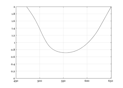
There is one adjustment I would like to make to the spectral colors.

% I would like to display spectral colors that are imilar in their
% brightness.  To adjust the overall luminance of the spectral values, I
% will scale the XYZ values of each spectral light by a function that is
% related to the Y value.  Remember that the Y value is correlated with
% brightness.  So, if we scale by the Y value, we can compensate a bit for
% brightness differences.

% Here is what I propose to use as a scale factor.

Yvalue = XYZ(:,2);
scaleFactor = (Yvalue + 0.4);

% Now, let's scale the rgb values. Pay attention to the fact that I am
% doing this scaling in the linear RGB space.  This calculation would be
% wrong if I did it on the frame buffer values, rather than the linear RGB
% intensities.

rgbSpectrum = rgbSpectrum*diag( 1 ./ scaleFactor);
rgbSpectrum = rgbSpectrum';

% Here is a plot of the scale factors I used to make the
% brightness of the wavelengths more nearly equal.

vcNewGraphWin;
plot(wavelength,1./scaleFactor,'k')
set(gca,'ylim',[0 2]), grid on

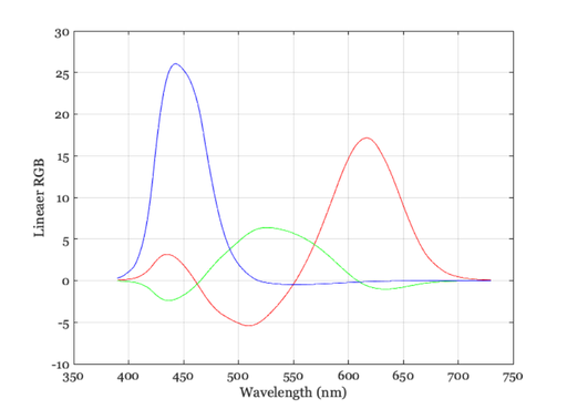
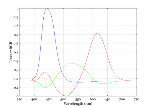
Here is a graph of the R,G and B values for each wavelength.

% The horizontal axis shows wavelength and the three colored curves show
% the linear intensity values needed for the phoshors.
vcNewGraphWin;
plot(wavelength,rgbSpectrum(:,1),'r', ...
    wavelength,rgbSpectrum(:,2),'g', ...
    wavelength,rgbSpectrum(:,3),'b')
grid on
set(gca,'xlim',[350 750]);
xlabel('Wavelength (nm)'); ylabel('Lineaer RGB');

Out of gamut colors

% Some of the RGB values are negative.  These are called "out of gamut" and
% cannot be displayed precisely.  There is no getting around this problem
% either for this example or in many real world applications. Some physical
% colors in the world simply cannot be displayed on conventional monitors,
% with three primaries.  This corresponds to the observation that in the
% color-matching experiment sometimes we must move one of the primaries to
% the other side of the field.

% There are many different suggestions (hacks) that people use to overcome
% the basic physical limitation of displays.  For our purposes, we can use
% a fairly simple compromise -- some of you may like it, others may not.
% That is the nature of this business.

% We can display these rgb values superimposed on a constant gray
% background.  By superimposing the spectrum on a constant background, we
% can both add and subtract RGB values.

% I propose that we use a gray background that is only as bright
% as the most negative rgbSpectrum value.

grayLevel = abs(min(rgbSpectrum(:)))
rgbSpectrum = (rgbSpectrum + grayLevel);

% And, we scale the RGB values in rgbSpectrum so they are as large as
% possible, but the sum of the background and these values will still be
% less than the maximum display value (1).

rgbSpectrum = rgbSpectrum/max(rgbSpectrum(:));

vcNewGraphWin;
plot(wavelength,rgbSpectrum), grid on
set(gca,'xlim',[350 750]);
xlabel('Wavelength (nm)'); ylabel('Lineaer RGB');

% Now, we correct for the display nonlinearities by presuming that we know
% something (which we don't) about your display. Here is the display gamma
% function relating a standard monitor frame buffer entries to the display
% intensities.

% load cMatch/hit489Gam

grayLevel =

    5.4240

Convert for the nonlinear DAC values

% Here is the function we use to convert the linear values in rgb to the
% frame buffer (DAC) values.
gTable = displayGet(d,'gtable');
DAC = lrgb2srgb(rgbSpectrum);

% To display the image, we sample every other wavelength value.  I am
% worried about running out of color map entries!
waveSamp = 1:2:size(DAC,1);
mp = DAC(waveSamp,:);
wavelength = wavelength(waveSamp);

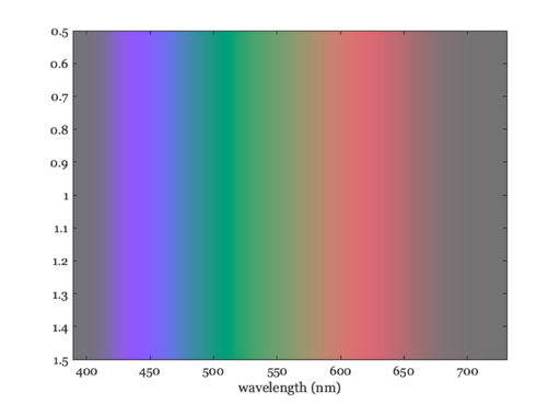
Show the image

% Create a linear ramp to show the color map values.
im = 1:size(mp,1);

% and show 'em
%
vcNewGraphWin;
mp = mp/max(mp(:));
colormap(mp);image(wavelength,1,im)
xlabel('wavelength (nm)')

% Notice that the color start to fade towards the end.  Why do
% you think that is?  Try varying some of the choices I made,
% such as the scaleFactor and the intensity of the gray
% background.

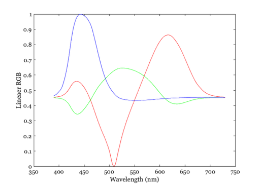
Here is a plot of the DAC values we ended up with.

vcNewGraphWin;
plot(wavelength, DAC(waveSamp,1),'-r',...
    wavelength, DAC(waveSamp,2),'-g',...
    wavelength,DAC(waveSamp,3),'-b')
set(gca,'xlim',[350 750]);
xlabel('Wavelength (nm)'); ylabel('Lineaer RGB');

% Notice that the overall saturation is quite limited by one part
% of the spectrum.  Perhaps if we didn't try to reproduce just
% that part of the image, or we adjusted just that part, we could
% obtain a more saturated overall appearance. Again, a design
% decision.

Published with MATLAB® R2024a