Illustrate a metameric matching and chromatic aberration

Metamerism is a fundamental insight of color science. In its principal scientific use, metamers are lights with different spectral power distributions that are visually indistinguishable.

People in industry also use metamerism to refer to the phenomenon that the same surface, scene under two different lights, does not appear the same.

This script describes the scientific analysis of metamers. We simulate a uniform field with D65 spectral power distribution and find a matching (metameric) LCD display output.

The two metameric lights are then used to create a bar pattern. We represent the bar pattern after optical blurring and then encoded by the human cone sensor array.

(c) Imageval Consulting, LLC 2012

Contents

ieInit

Create a uniform scene with a D65 spectral power distribution

uSize = 64;
uniformScene = sceneCreate('uniformd65',uSize);
sceneWindow(uniformScene);

Create a uniform field with a metameric spectral power distribution

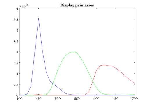
% The new spectrum is the weighted sum of the primaries of an LCD spectrum.
% The display primary intensities are chosen so that the LCD has the same
% effect as the D65 on the cone excitations.

% The mean LMS cone values of the original
lms     = sceneGet(uniformScene,'lms');
meanLMS = mean(RGB2XWFormat(lms));

% Load a display and use the display primaries as a set of basis
% functions for the metameric light.
d    = displayCreate('lcdExample');
wave = sceneGet(uniformScene,'wave');
displaySPD = displayGet(d,'spd',wave);

% These are the display primaries
vcNewGraphWin; plot(wave,displaySPD)
title('Display primaries')

% Now read the Stockman cone wavelength sensitivities
stockman = ieReadSpectra('stockmanEnergy',wave);
dW = wave(2)-wave(1);   % Delta Wavelength

% Solve for the weights on the display primaries that will produce the same
% absorptions in the cones as the D65 light.  Be careful to account for the
% wavelength sample spacing, dW.
%
%   meanLMS(:) = S'*(displaySPD*w)*dW
%
w = ((stockman'*displaySPD)\meanLMS(:))/dW;

%{
% The solution is pretty close
(stockman'*displaySPD*w*dW - meanLMS(:))/norm(meanLMS)
%}

metamer = displaySPD*w;

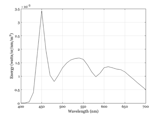
Plot the Stockman metamera

ieNewGraphWin;
plot(wave,metamer,'k-');
xlabel('Wavelength (nm)');
ylabel('Energy (watts/sr/nm/m^2)');
grid on;

%{
% Note: These original SPD is not an XYZ metamer. The Stockman and XYZ
% functions differ noticeably.  That is why the scene display has a bit of
% a difference!
disp(ieXYZFromEnergy(metamer',wave))
XYZ = sceneGet(uniformScene,'xyz');
disp(mean(RGB2XWFormat(XYZ)));
%}

Numerical check

%{
% The comparison projects of the SPDs of the metamers onto the Stockman
% cones.  The difference should be zero.  It is small, and I am not sure
% why it is not precisely zero.  I could probably do better.
disp(stockman'*(mSPD(:) - originalSPD(:)) / norm(originalSPD,2))

% Solution is pretty close.  The relative difference is better than 1 part
% in a million.  Not sure why it isn't perfect, though.
disp((stockman'*metamer(:) - stockman'*originalSPD(:))/norm(meanLMS))

%}

Create a new uniform scene with an SPD that is metameric to D65

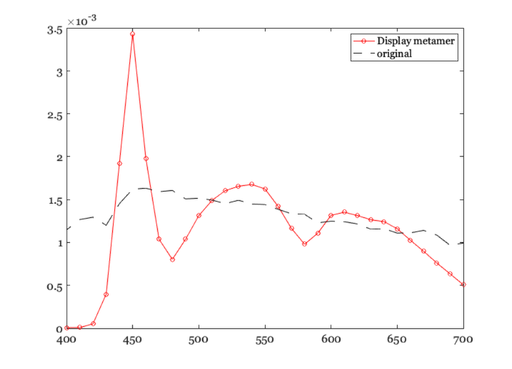
% We do this using the sceneSPDScale routine.  This multiplies the SPD in
% the scene by another SPD.  We use the metamer/originalSPD as the
% multiplier.

% Here is the original
originalSPD = sceneGet(uniformScene,'mean energy spd');

% Change the scene SPD to the metamer.
% Divide by the originalSPD and multiply by the metamer
skipIlluminant = false;
uniformScene2 = sceneSPDScale(uniformScene,(double(metamer(:))./double(originalSPD(:))),'*',skipIlluminant);
uniformScene2 = sceneSet(uniformScene2,'name','metamer');

% The metamer SPD
mSPD = sceneGet(uniformScene2,'mean energy spd');

% Why isn't the scaling more accurate?
% (mSPD(:) - metamer(:)) / norm(metamer)

% Make a plot comparing the metamer and the original mean energy (mn)
ieNewGraphWin;
plot(wave,mSPD,'-o',wave,originalSPD,'k--');
legend('Display metamer','original')

% Note that the color appearance on the screen differs between these two
% metamers.  That is because I did not implement a rendering algorithm
% based on human vision and the cones.  I used a method that is faster.  I
% am thinking of changing because, well, computers are now faster.
sceneWindow(uniformScene2);

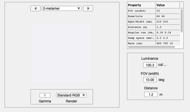
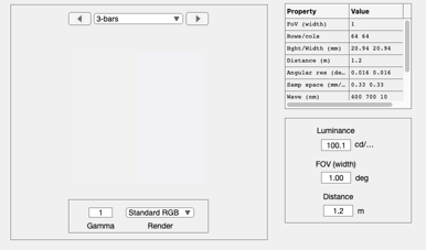
A spatial pattern with two metamers side by side.

% This will enable us to see the effect of optical blurring on the
% different spectral power distributions.

% Retrieve the SPD data from the two different uniform scenes.
height = 64; width = 32;
xwData  = sceneGet(uniformScene,'roi photons',  [8 8 width-1 height-1]);
xwData2 = sceneGet(uniformScene2,'roi photons',[8 8 width-1 height-1]);

% Combine the two data sets into one and attach it to a new scene
cBar = XW2RGBFormat([xwData; xwData2],height,2*width);
barS = sceneSet(uniformScene,'photons',cBar);

% Name it, set the FOV, and show it.
barS = sceneSet(barS,'name','bars');
barS = sceneSet(barS,'h fov',1);
sceneWindow(barS);

Compute the OI and show the SPD across a line in the image

if ~isempty(which('Lens'))

    % Notice that the optical image spectral irradiance varies across
    % the row. The LCD spectra are clearly scene at the positive
    % positions.  They are blurred a little onto the left side by the
    % optics.
    oi = oiCreate('wvf human');
    oi = oiCompute(oi,barS);

    midRow = round(oiGet(oi,'rows')/2);
    oiPlot(oi,'h line irradiance',[1,midRow]);
    title('1 cpd bar');
    oiWindow(oi);

Compute the sensor response for these half degree bars

    % Although the spd of the OI differs across the image the cone
    % absorptions are fairly constant across the horizontal line at
    % this spatial resolution.
    sensor = sensorCreate('human');
    sensor = sensorSet(sensor,'exp time',0.10);
    sensor = sensorSetSizeToFOV(sensor,1,oi);
    sensor = sensorCompute(sensor,oi);

    sz = sensorGet(sensor,'size');
    sensorPlot(sensor,'electrons hline',round([1,sz(1)/2]));
    sensorWindow(sensor);

end

END

Published with MATLAB® R2024a