Find linear transforms for blackbody illuminant corrections

We create pairs of scenes illuminated by different blackbody radiators. Then we find the best 3x3 transform between the different scenes.

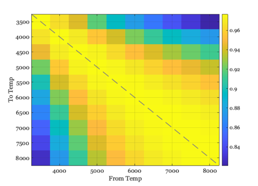
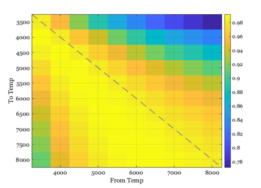
Then we measure how similar each of the large set of 3x3 transforms is to examples we found in another imaging project (L3).

NOTE: We used this script to assess the color transform for the L3 algorithm and the Buddha image. If you don't know what that means, just enjoy the table and images we produce below.

See also: blackbody, sceneAdjustIlluminant, sceneCreate, unitLength, RGB2XWFormat

HJ/BW Vistasoft Team, 2015

Contents

ieInit

Make a table of transforms that convert between these blackbody temperatures

% These are the blackbody color temperatures (degrees Kelvin)
bbRange = (3500:500:8000);
nbb = length(bbRange);
T = cell(nbb,nbb);   % This is the transform table

% We calculate using about 100 different reflectances
s = sceneCreate('reflectance chart');
wave = sceneGet(s,'wave');

Set the base illuminant as D65

for jj = 1:nbb   % To jj
    bb = blackbody(wave,bbRange(jj));
    s1 = sceneAdjustIlluminant(s,bb);

    XYZ1 = sceneGet(s1,'XYZ');
    XYZ1 = RGB2XWFormat(XYZ1);

    for ii = 1:nbb   % From ii

        bb = blackbody(wave,bbRange(ii));
        s2 = sceneAdjustIlluminant(s,bb);

        % ieAddObject(s); ieAddObject(s2); sceneWindow;

Find the linear transform

        XYZ2 = sceneGet(s2,'XYZ');
        XYZ2 = RGB2XWFormat(XYZ2);

        % Convert from this bb to the base
        % XYZ1 = XYZ2*T
        T{jj,ii} = XYZ2 \ XYZ1;  % From ii to jj

    end
end

Reconfigure the table into a matrix

% Put the 3x3 transforms in the columns
% Force them to be unit length vectors
transformList = zeros(9,nbb*nbb);
for ii=1:nbb*nbb
    transformList(:,ii) = unitLength(T{ii}(:));
end

comment = '3x3 transforms between different blackbody illuminants.  See s_colorILluminantTransforms.m';
fname = fullfile(isetRootPath,'data','lights','transformTable.mat');
save(fname,'bbRange','transformList','comment');

Buddha image transform

% This was the 3x3 transform we found for the Buddha image
B = [0.9245    0.0241   -0.0649
    0.2679    0.9485    0.1341
    -0.1693    0.0306    0.9078];

% C is the cosine of the angle between the transforms
B = unitLength(B(:));
C = transformList'* B(:);
C = reshape(C,nbb,nbb);

% Show the cosines as an image.
% N.B. We are not sure about the From/To labeling.  But this is
% consistent with the Buddha color becoming more yellow
ieNewGraphWin;
imagesc(bbRange,bbRange,C); colorbar
xlabel('From Temp'); ylabel('To Temp'); identityLine

ans = 

  Line with properties:

              Color: [0.5000 0.5000 0.5000]
          LineStyle: '--'
          LineWidth: 2
             Marker: 'none'
         MarkerSize: 6
    MarkerFaceColor: 'none'
              XData: [3250 8250]
              YData: [3250 8250]
              ZData: [1×0 double]

  Use GET to show all properties

Red flower transform

% This was the transform we found for a red flower image
F = [ 0.9570   -0.0727   -0.0347
    0.0588    0.9682   -0.1848
    0.0423    0.1489    1.2323];

% C is the cosine of the angle between the transforms
F = unitLength(F(:));
C = transformList'* F(:);
C = reshape(C,nbb,nbb);

% Show the cosines as an image.
ieNewGraphWin;
imagesc(bbRange,bbRange,C); colorbar
xlabel('From Temp'); ylabel('To Temp'); identityLine

ans = 

  Line with properties:

              Color: [0.5000 0.5000 0.5000]
          LineStyle: '--'
          LineWidth: 2
             Marker: 'none'
         MarkerSize: 6
    MarkerFaceColor: 'none'
              XData: [3250 8250]
              YData: [3250 8250]
              ZData: [1×0 double]

  Use GET to show all properties

Clean up the table

if exist(fname,'file'), delete(fname); end

Published with MATLAB® R2024a