seaborn.residplot

seaborn.residplot(data=None, *, x=None, y=None, x_partial=None, y_partial=None, lowess=False, order=1, robust=False, dropna=True, label=None, color=None, scatter_kws=None, line_kws=None, ax=None)

Plot the residuals of a linear regression.

This function will regress y on x (possibly as a robust or polynomial regression) and then draw a scatterplot of the residuals. You can optionally fit a lowess smoother to the residual plot, which can help in determining if there is structure to the residuals.

Parameters:

dataDataFrame, optional

DataFrame to use if x and y are column names.

xvector or string

Data or column name in data for the predictor variable.

yvector or string

Data or column name in data for the response variable.

{x, y}_partialvectors or string(s) , optional

These variables are treated as confounding and are removed from the x or y variables before plotting.

lowessboolean, optional

Fit a lowess smoother to the residual scatterplot.

orderint, optional

Order of the polynomial to fit when calculating the residuals.

robustboolean, optional

Fit a robust linear regression when calculating the residuals.

dropnaboolean, optional

If True, ignore observations with missing data when fitting and plotting.

labelstring, optional

Label that will be used in any plot legends.

colormatplotlib color, optional

Color to use for all elements of the plot.

{scatter, line}_kwsdictionaries, optional

Additional keyword arguments passed to scatter() and plot() for drawing the components of the plot.

axmatplotlib axis, optional

Plot into this axis, otherwise grab the current axis or make a new one if not existing.

Returns:

ax: matplotlib axes

Axes with the regression plot.

See also

regplot

Plot a simple linear regression model.

jointplot

Draw a residplot() with univariate marginal distributions (when used with kind="resid").

Examples

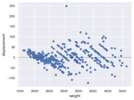
Pass x and y to see a scatter plot of the residuals after fitting a simple regression model:

sns.residplot(data=mpg, x="weight", y="displacement")

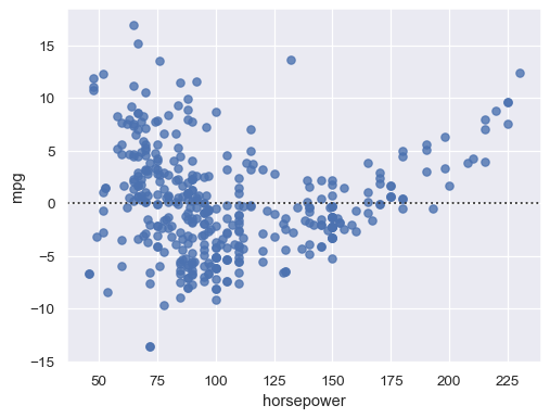
Structure in the residual plot can reveal a violation of linear regression assumptions:

sns.residplot(data=mpg, x="horsepower", y="mpg")

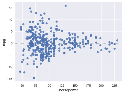
Remove higher-order trends to test whether that stabilizes the residuals:

sns.residplot(data=mpg, x="horsepower", y="mpg", order=2)

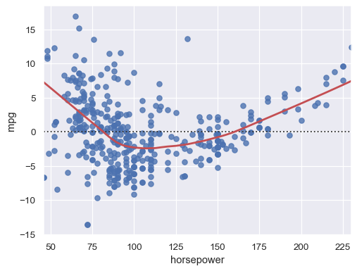
Adding a LOWESS curve can help reveal or emphasize structure:

sns.residplot(data=mpg, x="horsepower", y="mpg", lowess=True, line_kws=dict(color="r"))