William F.
Sharpe*
Stanford University
January, 1998
The last decade has seen the rapid growth of investment via mutual funds across the globe. This has led to a demand for simple measures of the performance of such funds. In the United States, the most popular is the "risk-adjusted rating" (RAR) produced by Morningstar, Incorporated. This measure differs significantly from more traditional ones such as various forms of the Sharpe ratio. This paper investigates the properties of Morningstar's measure. We show that the RAR measure has characteristics similar to those of an expected utility function based on an underlying bilinear utility function. This is of some concern, since strict adherence to a goal of maximizing expected utility with such a function could lead to extreme investment strategies. Next, we show that in practice, Morningstar varies one of the parameters of this function in a manner that frequently leads to results similar to those that would be obtained with the more traditional excess return Sharpe Ratio. Finally, we argue that neither Morningstar's measure nor the excess return Sharpe Ratio is an efficient tool for choosing mutual funds within peer groups when constructing a multi-fund portfolio --the ostensible purpose for which Morningstar's rankings are produced.
This paper analyzes the characteristics of the "risk-adjusted ratings" on which Morningstar, Incorporated bases its well-known "star ratings" and somewhat less well-known "category ratings", then compares these measures with more traditional mean/variance measures such as the excess return Sharpe ratio.
It is common for a mutual fund family to proudly advertise that one of its funds or possibly several funds have "received 5 stars from Morningstar". One study1 found that as much as 90% of new money invested in stock funds in 1995 went to funds with 4-star or 5-star ratings. While this may or may not be the correct figure today, few if any advertisements announce that a fund has received 1 star. For better or worse, Morningstar's risk-adjusted measures greatly influence U.S. investor behavior. Since they differ significantly from traditional risk-adjusted performance measures such as various forms of the Sharpe ratio, it is important to understand their strengths and limitations.
Mutual fund performance measures are typically based on one or more summary statistics of past performance. Measures that attempt to take risk into account incorporate both a measure of historic return and a measure of historic variability or loss. Since investment decisions only affect the future, the use of historic results involves an implicit assumption that the statistics derived from past performance have at least some predictive content for future performance. For example, a measure of average or cumulative return over some historic period may be assumed to provide information concerning expected return over some future period. Correspondingly, a measure of past variability or average magnitude of loss may be assumed to provide information about future risk or the likely loss over some future period.
While measures of historic variability can be useful for predicting future levels of risk, there is ample evidence that measures of average or cumulative return are at best highly imperfect predictors of expected future return. We leave questions of predictability for other papers. Our goal is to examine the properties of Morningstar's and other measures under the heroic assumption that statistics from historic frequency distributions are reliable predictors of corresponding statistics from a probability distribution of future returns. In particular, we seek to relate alternative performance measures to likely investment decisions on the grounds that one should attempt to select a performance measure that aligns well with the decision to be undertaken, even if the relationship between the past and the future is subject to a great deal of noise. Ultimately, of course, the goal is to use all relevant information to make unbiased forecasts of expected returns, risks, and any other relevant characteristics of future fund performance, then use such estimates to determine an optimal combination of investments in appropriate funds.
Our analysis of the Morningstar measures focuses on their key properties. The reader interested in empirical analyses of these and more traditional measures as well as the similarities and differences among them in practice will find a relatively extensive treatment in Sharpe [1997] .
We begin with a description of the computations used by Morningstar.
The Risk-adjusted Rating (RAR) for a fund is calculated by subtracting a measure of the fund's relative risk (RRisk) from a measure of its relative return (RRet):
RARi = RReti - RRiski
Each of the relative measures for a fund is computed by dividing the corresponding measure for the fund by a denominator that is used for all the funds in a specified peer group. Letting g(i) represent the peer group to which fund i is assigned:
RReti = Reti / BRetg(i)
RRiski = Riski / BRiskg(i)
where BRetg(i) and BRiskg(i) denote the bases used for the relative return and relative risk of all funds in the group in question.
Morningstar calculates RAR values taking load charges into account for purposes of determining its "star ratings". However, their newer "category ratings" omit load charges. The time periods utilized also differ. Four sets of star ratings are computed. The first three cover the last 3, 5 and 10 years, while the most popular (overall) measure is based on a combination of the 3,5 and 10-year results. In contrast, the category ratings cover only the last 3 years (36 months).
For simplicity, we describe only the calculations for the RAR values used for the category ratings. Sharpe [1997] provides considerable detail about the broader set of measures as well as a host of empirical analyses of their similarities and differences.
Morningstar's measure of a fund's return is the difference between the cumulative value obtained by investing $1 in the fund over the period and the cumulative value obtained by investing $1 in Treasury bills:
Reti = VRi - VRb
Thus if $1 invested in the fund would have grown to $1.50 in 36 months, assuming reinvestment of all distributions, while $1 invested in Treasury bills would, with reinvestment, have grown to $1.20:
Reti = 1.50 - 1.20 = 0.30, or 30%
Two steps are required to calculate the base to be used to calculate the relative returns for all the funds in a group. First, the returns for all the funds in the group are averaged. If the result is greater than the increase in value that would have been obtained with Treasury bills, the group average is used. Otherwise, the growth in value for Treasury bills is used. Thus:
BRetg(i) = max ( mean i in g(i) [Reti], VRb - 1)
Note that for the average value of Reti to be used, the funds must do at least twice as well as Treasury bills -- that is:
mean i in g(i) (VRi - 1) >= 2*(VRb - 1)
As we will show, the fact that BRetg(i) may have one of two distinct values makes it difficult to characterize the RAR measure in general terms.
To measure a fund's risk, Morningstar first computes the fund's excess return (ER) for each month by subtracting the return on a short-term Treasury bill from the fund's return. Next, all the positive monthly excess returns are converted to zeros. Finally, a simple mean is taken of the resulting "monthly losses" and the sign reversed to give a positive number2 Thus:
Riski = - meant ( mint [ERit , 0] )
The result is defined as a measure of the fund's "average monthly loss". More strictly, it is a measure of opportunity loss, where the foregone opportunity is investment in Treasury bills, and months in which there was an opportunity gain are counted as periods of zero opportunity loss.
The base used to calculate the relative returns for all the funds in a group is simply the average of all the risk measures for the funds in that group:
BRiskg(i) = meani in g(i) [Riski]
For purposes of calculating RARs, each fund is assigned to one (and only one) peer group. For its star ratings, Morningstar uses four such groups: domestic equity, international equity, taxable bond, and municipal bond. For its category ratings, peer groups are defined more narrowly. In mid-1997, for example, there were 20 domestic equity categories, 9 international equity categories, 10 taxable bond categories, and 5 municipal bond categories.
While Morningstar reports relative returns, relative risks and risk-adjusted ratings, most attention is focused on the "stars" and "category ratings" derived from the RAR values. To assign these measures, the RARs for all the funds in a peer group are ranked; funds falling in the top 10% of the resulting distribution are given 5 stars (or a category rating of 5), those in the next 22.5% get 4, those in the next 35% get 3, those in the next 22.5% get 2, and those in the bottom 10% get 1.
Most academic treatments of risk and return are based on the mean-variance approach developed in Markowitz [1952]. Markowitz argued that the desirability of a probability distribution of portfolio returns should be summarized using the first two moments: the expected return and the standard deviation of return (or its square, the variance of return). The ex post counterparts are the arithmetic mean return, which we will denote Mi for fund i and the standard deviation of historic returns, which we will denote Si.
For an investor who chooses only one mutual fund, the fund's return will equal his or her overall portfolio return. In this very special case, if the investor follows Markowitz' prescriptions, the expected utility of a portfolio invested solely in fund i can be written as:
EUi = Mi - rk* (Si2)
where rk is a measure of investor's k's risk-aversion -- that is, his or her marginal rate of substitution of mean return for variance of return. The goal of such an investor is to select the one fund for which this measure is the greatest, under the maintained assumption that historic returns are appropriate predictors of future returns.
While this type of expected utility function is widely used for optimization analyses, it is rarely chosen for ex post performance measurement. In part this is due to the fact that it only applies strictly when all an investor's funds are to be allocated to one single risky investment. Even more limiting, however, is the fact that in principle no universal measure of this type can be used by all investors. Rather, each investor must evaluate performance using a measure designed for his or her degree of risk aversion (rk).
In an important contribution to investment theory, Tobin [1958] showed that combining a riskless investment with a risky one provides an opportunity set in which expected excess return is proportional to return standard deviation. This implies that an investor able to borrow or lend at a given rate and who is planning to hold only one mutual fund plus borrowing or lending should select the fund for which the ratio of expected excess return to standard deviation is the highest. This ratio is generally termed the Sharpe ratio, based on its introduction in Sharpe [1966]. As shown in Sharpe [1994], the key properties of the original measure apply more broadly to any "zero-investment strategy" such as that given by the difference between the returns on any two investments. To avoid confusion, we refer to the measure based on excess returns as the excess return Sharpe ratio (ERSR). Letting Rbt represent the return on a riskless security, the excess return Sharpe Ratio for fund i is:
ERSRi = meant (Rit - Rbt) / stdevt (Rit - Rbt)
Ex ante, Rb is a fixed constant, so that:
ERSRi = (Mi - Rb) / Si
Ex post, the more complete formula is typically employed to account for any variation in Rb.
The goal of an investor able to borrow or lend at a fixed rate but planning to hold only one risky mutual fund is to select the fund with the greatest ex ante ERSRi since a strategy employing it with the appropriate amount of leverage can provide the greatest possible expected return for any desired level of risk As with other measures, of course, selection of a fund with the highest ex post excess return Sharpe ratio is only appropriate under the maintained assumption that the historic return distribution is a good predictor of the future probability distribution.
Excess return Sharpe ratios are often used as measures of mutual fund performance, partly because they are less limited in applicability than mean variance expected utility measures. Importantly, under the assumptions on which the argument is based, the fund with the greatest Sharpe ratio is the best for any investor, regardless of his or her degree of risk aversion. In this sense, the measure is universal. Strictly, of course, the ratio is suitable only for cases in which an investor plans to invest funds in a single risky asset plus (possibly) borrowing or lending. Thus it is slightly more general (two investments rather than one), but still potentially inappropriate for a more typical portfolio involving multiple risky funds.
As shown, a fund's RAR is the difference between two relative measures:
RARi = [ Reti / BRetg(i) ] - [ Riski / BRiskg(i) ]
Rearranging slightly gives:
RARi = (1 / BRetg(i) ) * [ Reti - ( BRetg(i) / BRiskg(i) ) Riski ]
Note that both the first and second parenthesized expressions are the same for all the funds in a given group. Since the first term must be positive, both the rankings of funds within a group and the relative magnitudes of their ratings will be unaffected if this term is omitted. Denoting the second parenthesized expression as kg(i) gives a re-scaled RAR of the form:
RRARi = Reti - kg(i) * Riski
It is tempting to interpret this modified function as a measure of the expected utility of fund i for an investor with a risk aversion of kg(i), where risk aversion is a measure of the investor's marginal rate of substitution of Reti for Riski. Under this interpretation, kg(i) would represent the risk aversion of all investors who select funds in the group in question. We address the relevance of such an assumption later. For now we take RRAR as a measure of expected utility.
Sharpe ratios use standard statistics from a frequency distribution of differential returns. For example, the first two moments of the probability distribution of next month's excess return might be assumed to be similar to the same moments from the frequency distribution of the last 36 months' excess returns. Importantly, the same time period (e.g. monthly) is used for both statistics.
Morningstar's risk measure has a similar character. Each monthly loss is given the same weight, with the average value presumably used as a surrogate for the expected value of next month's loss. However, the measure of return is the difference between two cumulative values taken over the complete historic period. The properties of such a statistic are complex, since it represents the difference between two value relatives, each of which can be considered to equal the result obtained by raising [1 plus the geometric mean return] to the T'th power, where T is the number of months in the overall period. Since the geometric mean of a series of returns is a function of both the arithmetic mean and the variance of the series, the resulting return measure includes aspects of both return and risk.
Among other things, this makes the statistical properties of Morningstar's measure highly complex, seriously compromising the analyst's ability to estimate likely ranges of future performance, given historic results. This contrasts with the Sharpe ratio, which is a simple transform of the standard t-statistic for measuring the statistical significance of the difference between a realized mean value and zero and hence easily used in this manner.
We explore further implications of Morningstar's calculation in greater detail below. For now, we consider a modification that would make the RAR measure internally consistent. In particular, we use as a measure of return the difference between the fund's arithmetic mean monthly return and the arithmetic mean return on Treasury bills; we also modify the procedure used to calculate the relative return base accordingly:
MRARi = MReti - mkg(i) * Riski
where :
MReti = meant (Rit - Rbt)
In this measure, mkg(i) is the marginal rate of substitution of mean monthly excess return for mean loss, given by:
mkg(i) = MBRetg(i) / BRiskg(i)
where:
MBRetg(i) = max ( meani in g(i) [MReti], meant [Rbt] )
Except in extreme cases, the relative MRARi values for the funds within a peer group will be similar to those obtained using Morningstar's actual procedures (that is, the corresponding RRARi or RARi values). In the following analysis, we assume that MReti, BRetg(i) and kg(i) are computed using arithmetic monthly mean values. This allows us to obtain precise analytic results. Fortunately, the main qualitative conclusions apply as well to the more complex measures utilized by Morningstar.
Consider an investor with a Von Neuman-Morgenstern utility function of the form:
U = a* (Ri - Rb) if Ri <= Rb, and
U = (Ri - Rb) if Ri > Rb
where Ri is the return on fund i, Rb is the return on treasury bills, and a is a constant greater than one.
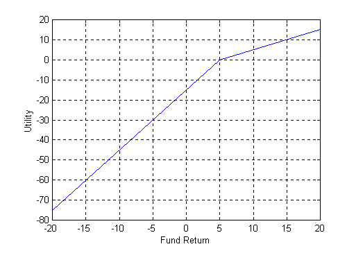
An example of such a function in which Rb=5% and a= 3 is shown in Figure 1. As can be seen, it is composed of two linear segments, with a greater slope to the left of Rb than to the right. Such a function exhibits risk-aversion in the large, since the loss in utility associated with a return below Rb is greater than the gain in utility associated with a return equally far above Rb. However, within return ranges that lie wholly above or wholly below Rb, the function is linear and thus reflects risk-neutrality.
Figure 1: A Bilinear Utility Function
A bilinear function of this sort captures one of the three salient features of the prospect theory of decision-making under uncertainty derived by Kahneman and Tversky [1979] from observation of choices made by subjects in experimental settings. An individual with such a function experiences loss-aversion, where loss is measured from a reference point determined by the current riskless rate of return Rb. More precisely, the function can be said to reflect opportunity loss aversion, with the value of the parameter a providing a measure of the degree of such aversion and the riskless rate acting as the reference point or alternative investment opportunity.
Now consider an investor with a bilinear utility function who wishes to determine the expected utility of a given mutual fund over a future period.
To begin, we rewrite the formula for the utility function as:
U = Ri - Rb + [(a - 1) *(Ri - Rb) if Ri <= Rb and 0 otherwise]
The expected value of U will thus be:
E(U) = E( Ri - Rb ) + (a - 1)* E ( Li)
where:
Li = Ri - Rb if Ri <= Rb, and
Li = 0 if Ri > Rb
Note that Li is exactly equal to Morningstar's monthly loss figure..
Let there be T possible future returns, each equally likely to be realized. Then the expected values are simply arithmetic means, and:
E(U) = mean ( Ri - Rb ) + (a - 1)* mean( Li)
Substituting historic excess returns for future returns gives a measure that would be precisely equal to Morningstar's RAR if the latter used arithmetic mean monthly excess returns for its return calculations. Since the differences due to this disparity are likely to be small, in form, Morningstar's RAR measure is highly similar, if not identical, to that that would be chosen by an investor who wishes to maximize a bilinear utility function but has decided to invest in only one mutual fund.
Compare the equation for expected utility with our modified version of Morningstar's RAR measure:
MRARi = Reti - kg(i) * Riski
Thus it is approximately true that:
a = 1 + kg(i)
Since kg(i) is positive, the investor will exhibit opportunity loss aversion, with the magnitude of aversion greater, the larger is kg(i).
While the bilinear utility function has at least one attractive property, on closer examination it can be shown to imply extreme investment choices under plausible circumstances, as we now show.
Consider a strategy in which a proportion of an investor's wealth equal to x is placed in risky fund i and a proportion equal to (1-x) is placed in a riskless asset. The mean and variance of the strategy's excess return will be given by x*Mi and x*Si, respectively. Since both measures are linear in scale, their ratio is scale-independent. Thus the excess return Sharpe ratio for the strategy will equal that of the fund itself. Indeed, it is the fact that Sharpe ratios are scale-independent that makes them attractive as measures of performance.
For such strategies, both of Morningstar's measures are also proportional to scale. Recall that:
Reti = VRi - VRb
Letting TRi and TRb represent the total compound return for fund i and bills, respectively, over the period covered:
Reti = ( 1 + TRi ) - ( 1 + TRb ) = TRi - TRb
For a strategy in which x is invested in fund i and (1-x) in Treasury bills:
Retx = [ x*(1 + TRi ) + ( 1-x)*( 1 + TRb )] - (1 + TRb) = x*(TRi - TRb) = x*Reti
A similar relationship holds for the average loss measure. In months for which Ri <= Rb:
L = x*(Ri - Rb)
while for months for which Ri > Rb:
L = 0 = x*0
Hence for the strategy in which x is invested in fund i and (1-x) in Treasury bills:
Riskx = x * Riski
The fact that both Morningstar's measures are proportional to scale implies that by combining a risky fund with borrowing or lending, an investor can attain any point on a linear opportunity set in Retx-Riskx space. Faced with such a tradeoff, what choice will be made by an investor with a bilinear utility function?
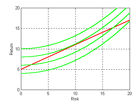
Figure 2 shows three possible outcomes. In each case, the opportunity set is shown by the red line. The green lines are representative iso-expected utility lines . All combinations of risk and return along any such line provide the same expected utility, with higher lines representing greater expected utility than lower lines. Each investor's objective is to find the feasible point (on the red line) with the highest expected utility (on the highest attainable green line). The three figures represent investors with different degrees of risk aversion. The investor in the left-hand panel is the most risk averse; the investor in the right-hand panel is the least risk averse;the investor in the middle panel has an intermediate degree of risk aversion.
Figure 2: Investment Choice for Three Investors with Bilinear Utility Functions
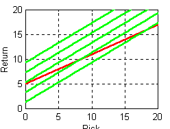
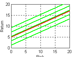
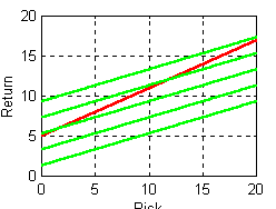
Note that for two out of the three investors the optimal choice is an extreme one. The conservative investor invests solely in Treasury bills, while the aggressive investor puts as much as possible in the mutual fund, borrowing to the maximum allowable limit. Only for an investor with risk aversion precisely equal to the available risk-return tradeoff is any interior strategy optimal, and any such investor is totally indifferent to the degree of leverage involved.
Such choices are clearly inconsistent with the observed behavior of the vast majority of investors, calling into serious question the assumption that investors have utility functions as simple as that of the bilinear form. The problem is mitigated slightly in settings in which many investment options are available and multiple funds may be selected. However, even in such cases, the efficient opportunity set is likely to be close to linear, leading to very similar results.
Note that these objections apply as well to a function in which expected utility is a linear function of mean (Mi) and standard deviation (Si). The problem does not arise, however, using the Markowitz formulation in which expected utility is a linear function of mean and variance, since the implied iso-expected utility curves increase at an increasing rate in mean/standard deviation space. As shown in Figure 3, such preferences lead to interior investment choices, even when the efficient portion of the opportunity set is linear.
Figure 3: Investment Choice for an Investor with a Mean-Variance Utility Function
While Morningstar's RAR measure differs considerably from a utility function based on a fund's mean and variance of return, it is likely to be well approximated by a function of these more traditional measures.
To begin, consider Reti. It is the difference between the value relative for the fund and that for Treasury bills. But the value relative over T periods will equal one plus the geometric mean return (G) to the T'th power. Thus
Reti = ( 1 + Gi) T - (1 + Gb)T
A close approximation for the geometric mean of a series is given by subtracting one-half the variance from the arithmetic mean. Thus:
Reti = ( 1 + Mi - Si 2 / 2 ) T - (1 + Mb - Sb2 / 2)T
As can be seen, Morningstar's return measure incorporates aspects of both mean return and risk (standard deviation of return), with Reti increasing in Mi and decreasing in Si. Given knowledge of Mi and Si, one can clearly obtain a good estimate of Reti.
The situation is not as clear-cut for Riski. In general it will depend on both the shape of the return distribution and its moments. Letting prx be the probability of state of the world x and ERix the excess return on fund i in state x, the expected loss (Riski) for fund i is defined as:
Riski = - sumx [ prx*minx (ERix ,0) ]
Consider now the situation in which the mean and variance of the distribution of excess returns are sufficient statistics to identify the entire distribution. This is the case, for example, if returns are normally distributed. Under this assumption:
Riski = f [ Mi-Rb, Si ]
since Mi-Rb is the mean of the excess return distribution and Si is its standard deviation (assuming that Rb is known).
Using a relationship given in Triantis and Hodder [1990], it can be shown3 that for a normal distribution:
Riski = f [ Mi-Rb, Si ] = Si * n(-z) - (Mi - Rb) * N(-z)
where:
z = ( Mi-Rb ) / Si
Here, n(z) denotes the standard normal density function while N(z) denotes the standard cumulative normal. 3.
Empirical evidence given in Sharpe [1997] indicates that monthly return distributions for diversified mutual funds may be sufficiently close to normal to make this approximation quite accurate
If both Riski and Reti are well approximated as functions of Mi and Si, then RARi will be also.
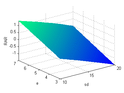
Figure 4 shows the relationship between RAR and various combinations of e (expected annual excess return) and sd (standard deviation of annual excess return) using the approximations given above for a case in which the riskless rate of interest is 5% per year, the holding period is 3 years, and the peer group has an average excess return of 5% and a standard deviation of 15%. As can be seen, the relationship is monotonic and very close to linear in the region shown, which includes likely combinations for popular investment strategies.
Figure 4: RAR as a Function of Expected Excess Return and Standard Deviation
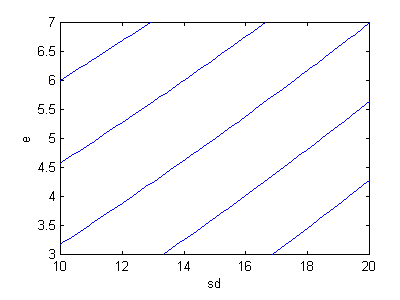
The high degree of linearity of the relationship in Figure 4 can be seen more clearly in Figure 5, which shows a few of the associated iso-RAR curves. Clearly an investor who wishes to maximize RAR is likely to select an extreme solution unless the opportunity set is highly non-linear.
Figure 5: Iso-RAR Curves
Recall that a portfolio is said to be mean-variance efficient if it provides the maximum possible mean for a given level of variance and the minimum possible variance for a given level of mean. Equivalently, fund A is said to be inefficient if there exists another fund B with (1) the same expected return but less risk, (2) the same risk but more expected return, or (3) less risk and more expected return. With functions such as those shown in Figures 4 and 5, in each such case, fund B would also have a higher RAR value than fund A if the approximations held. Thus it would be appropriate to exclude from consideration portfolios that are inefficient using the mean-variance criterion even if the ultimate goal were to select a portfolio with the largest possible RAR value.
These relationships imply that the key differences between Morningstar's measures and those used in more traditional mean-variance analyses concern (1) the use of a linear combination of a return measure and a risk measure, rather than a ratio of the two and/or (2) the use of risk per se rather than risk-squared in the linear measure. The use of a multi-period value relative and a measure of average loss is thus of secondary importance in terms of implications for fund selection.
These results provide an illustration of our earlier assertion that Morningstar's actual RAR calculations give implications for investment choice very similar to those obtained using the simpler modified (MRAR) measure. Moreover, they suggest that if monthly returns are close to normally distributed, a choice based on a RAR measures will differ from one based on the use of a traditional mean-variance approach only in the selection of an extreme point on the mean-variance efficient frontier rather than an interior point on that same frontier. This is unfortunate since a preference for extreme risk-return combinations is inconsistent with investor behavior. In effect, the RAR measure assumes that an investor's marginal rate of substitution of expected return for risk is the same, no matter what the level of his or her portfolio's return or risk. This is inconsistent with observed behavior -- both in this context and in more general cases involving choices among competing alternatives.
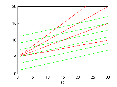
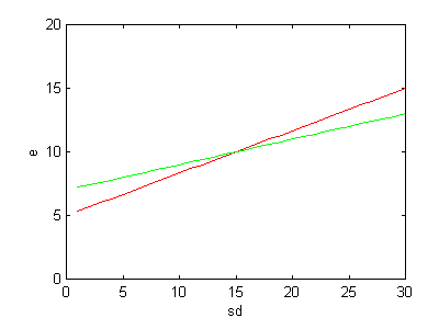
Clearly, there are conceptual difference between rankings of funds based on RAR values and excess return Sharpe Ratios. This can be seen in Figure 6, which shows selected iso-excess return Sharpe Ratio lines (iso-SR for short) in red and selected mean-variance approximations of iso-RAR curves in green.
Figure 6: Iso-Excess Return Sharpe Ratio Lines and Approximate Iso-RAR Curves
To assess the likely magnitudes of such differences, consider a selected mutual fund, X and the iso-RAR and iso-SR lines on which it lies. Figure 7 shows a case in which fund X has an expected return of 10% and a standard deviation of 15%.
Now consider the set of all funds that are better than X based on the RAR criterion. They will lie above the green line in Figure 7. Similarly, the set of all funds that are worse than X based the RAR criterion will lie below the green line. On the other hand, funds that are better than X based on the ERSR criterion will lie above the red line and those that are worse will lie below the red line.
Figure 7: The Iso-SR and Iso-RAR Lines for a Single Fund
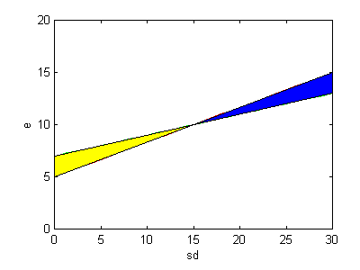
Obviously, the sets of funds rated better or worse than X may be different, depending on the criterion used. However, the differences may be relatively few. Figure 8 shows the regions in which the criteria give different results. Any fund plotting in the blue area will have a higher RAR than fund X but a lower ERSR. Any fund plotting in the yellow area will have a lower RAR than fund X but a higher ERSR. However, for all funds that plot above both lines or below both lines, the criteria will lead to the same conclusion. In general, the closer the slopes of the two lines, the fewer will be the disparities in rankings between the two criteria.
Figure 8: Regions in Which the SR and RAR Criteria Conflict
Now, recall the procedures used to compute Morningstar's RAR measures. As we have shown, the slope of the iso-RAR curve is given by the ratio of the return base to the risk base. If the period used for the computation has been one in which the average return for the funds in the relevant peer group has been sufficiently high (greater than two times the return on Treasury bills), the return base will equal the mean excess return for the funds in the peer group. In every case the risk base is the mean risk for the funds in the peer group. Let a fund (A) have a mean excess return and standard deviation of return equal, respectively, to the corresponding average value for all the funds in its peer group. This implies that under such conditions, by construction, the mean-variance approximation to the iso-RAR line for fund X will be coincident with the iso-SR line for the fund.
In such circumstances, the sets of funds that are better and worse than fund A will be the same, no matter which criterion is used. The same can be said about any fund that plots on fund A's iso-SR (and iso-RAR) line -- that is, any fund with the same ERSR as a fund with the average risk and return for the peer group. In practice, funds are likely to cluster reasonably closely around this line. Hence we might well expect that for peer groups with good average historic performance, rankings based on Morningstar's RAR measure might be relatively similar to those based on the more traditional excess return Sharpe Ratio.
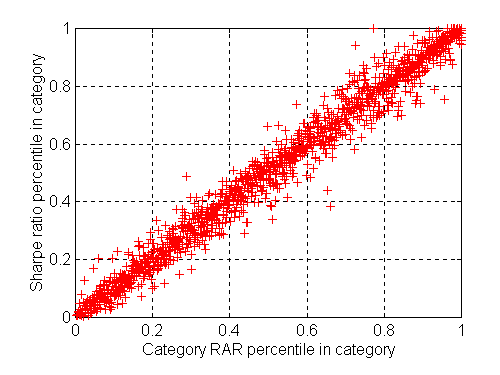
Figure 9, taken from Sharpe [1997], shows that this can indeed be the case. Each point represents the ranking of a one of 1,286 diversified equity funds within its category peer group, based on performance from 1994 through 1996. The correlation coefficient was 0.986, showing that despite substantial differences in computational procedures, Morningstar's approach and the simpler excess return Sharpe Ratio do indeed give similar results in times such as the 1994-1996 period of relatively high returns for U.S. equity funds.
Figure 9: Rankings Based on Morningstar's Category RARs and Excess Return Sharpe Ratios
While these results are quite striking, it is important to note that they apply to a situation in which returns were high and Morningstar's procedure therefore utilized the mean returns of the peer groups for the return bases in the calculations. Since ex post returns are used for the performance measures, there can be situations in which the average return for a peer group is small or even negative. In such cases, Morningstar sets the return base at the level obtained by Treasury bills. This may well lead to a greater disparity in rankings based on the Morningstar and Sharpe Ratio measures.
Figure 10 shows an extreme version of such a situation. Here, both funds X and Y have performed poorly. However, fund Y had a better (algebraically greater, or less negative) excess return Sharpe Ratio than fund X, as shown by the fact that it lies on a higher iso-SR (red) line. On the other hand, Morningstar's RAR measure assigns a better rating to fund X than to fund Y, since X provided a better average return and a lower risk, leading the fund to plot on a higher iso-RAR (green) line.
Figure 10: Performance of Two Funds in Bad Times
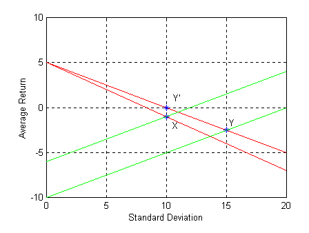
This example makes very clear the differences in the questions that the two measures attempt to answer. We have argued that the RAR measure is best seen as an attempt to determine the best single fund on the assumption that only one fund is to be held in the investor's portfolio. In this context, X was certainly better (here, less bad) than Y. Moreover, this would be true for any (positive) degree of investor risk-aversion (slope of the iso-RAR lines). However, this is not the setting for which the excess return Sharpe Ratio was developed. It is intended for situations in which an investor can use borrowing or lending to achieve his or her desired level of risk. In this context, the excess return Sharpe Ratio gives the more appropriate answer. An investor who desired a level of risk of, say 10% would have held either fund X or a 50/50 combination of fund Y and lending at the riskless rate (here, 5%). The latter strategy, shown by point Y' in Figure 10, was clearly better than investment in fund X, as shown by its greater excess return Sharpe Ratio.
Morningstar's measure is best suited to answer questions posed by an investor who places all his or her money in one fund. The excess return Sharpe Ratio is best suited to answer questions posed by an investor who allocates money between one fund and borrowing or lending. Neither type of investor should be interested in ranking funds within peer groups -- indeed such rankings conceal information about the relative magnitudes of the underlying variables that is crucial for such an investor.
Why then does Morningstar present its risk-adjusted ratings in terms of rankings of funds within peer groups? The only plausible answer is that investors are assumed to have some other basis for allocating funds across peer groups and plan to use Morningstar's rankings as at least an important input when deciding which fund or funds to choose from each peer group. In such a situation, neither Morningstar's measure nor the excess return Sharpe Ratio is an appropriate performance measure. The reason is simple. When evaluating the desirability of a fund in a multi-fund portfolio, the relevant measure of risk is its contribution to the total risk of the portfolio. This will depend on the fund's total risk and, more importantly, in most cases, on its correlation with the funds in the remainder of the portfolio. Neither the Morningstar RAR measure nor the excess return Sharpe Ratio incorporates any information about such correlation. Excessive reliance on either measure in such a decision process could seriously diminish the effectiveness of the resulting multi-fund portfolio.
There are some very special cases in which a different single measure of fund performance may be useful when constructing an optimal multi-fund portfolio. For example, Sharpe [1994] shows that the Selection Sharpe Ratio, based on the difference between a fund's return and that of an appropriate asset class benchmark, may be used if long and short positions in asset classes can be taken as needed. However, the preconditions for this special case may not be met in many cases, and even if they are, there can be significant differences between rankings based on excess return Sharpe Ratios and Selection Sharpe Ratios. Given the relationships between RARs and excess return Sharpe Ratios, rankings based on Selection Sharpe Ratios will also differ considerably from those based on RARs.
In many if not most cases, the use of any procedure for ranking funds within peer groups, followed by selection of one or more funds from each of several peer groups based on such rankings, is likely to be suboptimal, and possibly highly suboptimal.
We have shown that Morningstar's RAR measure has a number of drawbacks. It is complex, with poor statistical qualities. More importantly, it fails to capture an important aspect of investor preferences -- increasing aversion to risk -- and the resulting desire for portfolios that are neither the least or most risky available. Fortunately, the inherent disadvantages are mitigated to a considerable extent by Morningstar's practice of adjusting the risk-aversion implicit in the measure to equal the ratio of return to risk for each peer group over the specific period covered, although this adjustment is made only in part if the peer group performance has been modest or poor. While this procedure makes the measure even more time and sample-dependent, it has the advantage of aligning rankings rather well with those that would be obtained using the more familiar, less complex and statistically more straightforward excess return Sharpe Ratio.
Given a choice between Morningstar's RAR measure and the excess return Sharpe Ratio, the evidence would seem to favor the latter. However, a more appropriate choice would involve either a different performance measure or none at all. If it is possible to costlessly separate fund selection from asset allocation by taking long and short positions in index funds representing "pure asset plays", funds may usefully be evaluated based on their projected Selection Sharpe Ratios. Such measures take into account only a fund's non-asset related expected return and risk. Typically, rankings based on selection Sharpe Ratios will differ considerably from those based on Morningstar's measures or excess return Sharpe Ratios. So of course will the resulting preferred portfolios.
While it is tempting to conclude that investors constructing multi-fund portfolios should shift their focus from performance measures based on total or excess return to those based on differential or relative-to-benchmark return, such is not our ultimate counsel. The conditions under which the Selection Sharpe Ratio is appropriate are stringent and unlikely to hold for a typical investor. Rather than continue the search for the ideal universal performance measure it is preferable to return to basics. Markowitz taught us that portfolios should be constructed taking into account the best possible estimates of all relevant future risks and returns. This is as true for portfolios of mutual funds as it is for portfolios of individual securities. Asset allocation exercises, followed by selection of funds within peer groups based on simple rankings, are easy but may lead to inefficient overall portfolios. A better approach takes into account the complexity involved in such decisions. The key information an investor needs to evaluate a mutual fund includes (1) its likely future exposures to movements in major asset classes, (2) the likely added (or subtracted) return over and above a benchmark with similar exposures, and (3) the likely risk vis-a-vis that benchmark. Efforts should be devoted to obtaining the best possible estimates for future values of these key ingredients, then using them optimally to determine efficient portfolios.
*. The author would like to thank John Watson of Financial Engines, Inc. for suggestions and comments on an earlier draft.
1. Described in Damato1996
2. For the calculations used by Morningstar, it makes no difference whether the sign is reversed, due to the subsequent division by the risk base, which is an average of all the risk numbers. However, for ease of interpretation, we reverse the sign so that a smaller absolute value of risk will be considered more desirable than a larger absolute value (as with standard deviation).
3. Function f was obtained by integrating over negative values of the excess return, taking into account the relationship shown in equation (A1) in Triantis and Hodder [1990].
Markowitz, Harry, "Portfolio Selection," Journal of Finance, March 1952, pp. 77-91
Sharpe, William F., "Mutual Fund Performance," Journal of Business, January 1966, pp. 119-138.
Sharpe, William F., "The Sharpe Ratio," Journal of Portfolio Management, Fall 1994.
Sharpe, William F., Morningstar's Performance Measures, 1997
Kahneman, Daniel and Amos Tversky, "Prospect Theory: An Analysis of Decision Under Risk," Econometrica, XXXXVII (1979): pp. 263-291.
Triantis, Alexander J. and James E. Hodder, "Valuing Flexibility as a Complex Option," The Journal of Finance, Vol. XLV No. 2, June 1990, pp. 549-564.