This file is part of scl, a control and simulation library for robots and biomechanical models.scl is free software; you can redistribute it and/or modify it under the terms of the GNU Lesser General Public License as published by the Free Software Foundation; either version 3 of the License,or (at your option) any later version.
Alternatively, you can redistribute it and/or modify it under the terms of the GNU General Public License as published by the Free Software Foundation;either version 2 of the License,or (at your option) any later version.scl is distributed in the hope that it will be useful, but WITHOUT ANY WARRANTY;without even the implied warranty of MERCHANTABILITY or FITNESS FOR A PARTICULAR PURPOSE. See the GNU General Public License for more details. You should have received a copy of the
GNU Lesser General Public License and a copy of the GNU General Public License along with scl. If not, see <http://www.gnu.org/licenses/>.
\file Math_RPPBot.nb
Created on : July 9,2012
Author : Samir Menon<smenon@stanford.edu>
Control tutorial : RPPBot
The RPP robot has 3 degrees of freedom, revolute-prismatic-prismatic and can position its hand in 3D cartesian coordinates xyz, or can orient its hand in 1D rotational (z-axis) coordinates.
Here, we will develop control equations for the RPPBot. The equations will allow joint space dynamic control as well as operational space dynamic control. The RPP bot has 3 dof and also has a 3 dof range space and so the controllers will both be 3 dimensional.
Helper Functions
In[1]:=
![]()
Computing Kinematics and Dynamics
The generalized coordinates : q
The gen coords are one possible minimal set of variables that are necessary and sufficient to describe the configuration of the robot. By
convention, we shall call these 'q'. The generalized velocities, and accelerations as a consequence, are dq and ddq.
For RPPBot, a suitable set of generalized coordinates is one joint angle and two joint positions.
In[2]:=
![]()
The Forward Transformation Matrices
The first step to compute the control equations is to figure out coordinate transformations from a universal, stationary "origin" frame to the robot' s links. These transformations are functions of the generalized coordinates and are updated as the robot moves. They allow us to compute the position of different points on its links (like the link centers of mass), and are used extensively in any controller.
In[3]:=
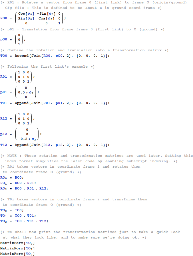
Out[18]//MatrixForm=

Out[19]//MatrixForm=

Out[20]//MatrixForm=

Center of Mass Positions and Jacobians
COM Mass/Inertias For RPP - Bot wrt. their respective link frames. We will compute Jacobians in the origin' s frame, and so will move these vectors to the origin' s frame.
In[21]:=
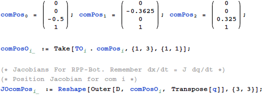
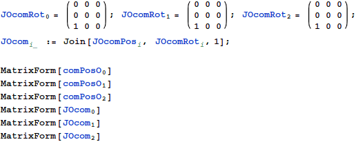
Ok. So we have the frame positions. But if you recall rigid body dynamics, the configuration of a rigid body also requires the orientation. But a Jacobian must relate the generalized velocities to position and rotational velocities.
This is where things get hairy. Though a rigid body has three rotational degrees of freedom, there are no three variables that can completely describe the set of its rotations as well as their inverses. Storing the orientation position "requires" four variables with their vector norm constrained to 1 (ie. a vector on the surface of a 4D hypersphere).
However, storing the orientation rotational velocities require only three variables. We shall use this fact to compute the rotational part of the Jacobian by directly
computing the linear map from end-effector rotations to generalized coordinates.
In[24]:=
Out[26]//MatrixForm=
![]()
Out[27]//MatrixForm=
![]()
Out[28]//MatrixForm=
![]()
Out[29]//MatrixForm=

Out[30]//MatrixForm=

Out[31]//MatrixForm=

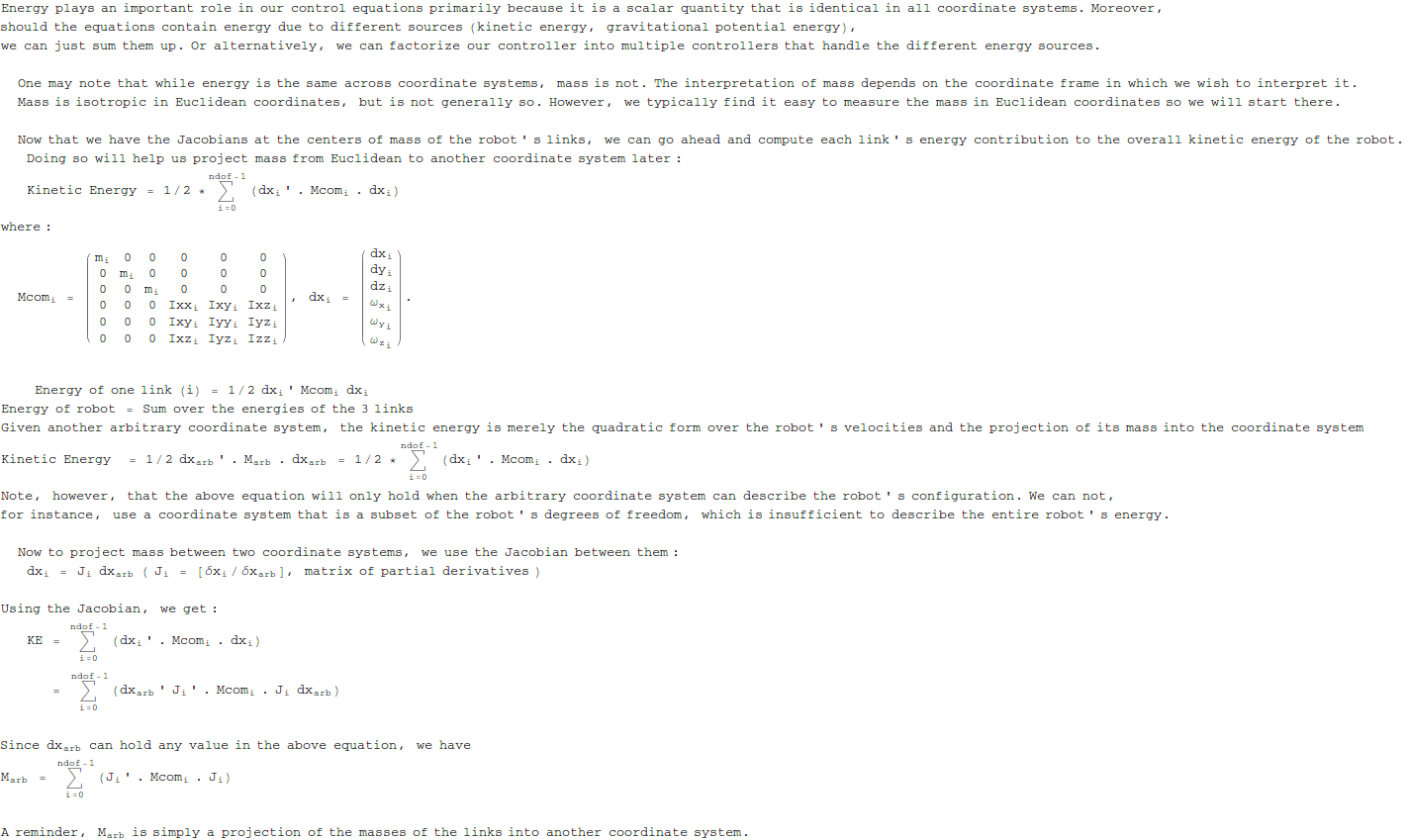
Using Energy Equivalence to Determine Mass In Arbitrary Coordinates
In[32]:=
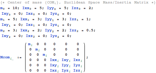
Mass in the Generalized Coordinates
Using the earlier equations we shall project mass into the generalized coordinates. Doing so will help us build our generalized coordinate controller.
Since dx = J dq, we can use our earlier energy equivalence equations, to get a notion of mass in the generalized coordinates :
1/2 dq' Mgc dq = 1/2 ![]()
We use this relationship to derive Mgc from the M_i of the links at their centers of mass. dq is arbitrary. So for the equations to hold, we must have :
Mgc = ![]()
In[39]:=

Out[40]//MatrixForm=
![]()
Out[41]//MatrixForm=

Potential Energy Equivalence and Generalized Gravity
The next step is to model the gravitational field :
The work done against gravity is the same in all coordinate systems,
and we shall use this to project the gravitational field into our generalized
coordinates.
![]() . δq =
. δq = ![]()
![]() . δq =
. δq = ![]() ....[δx = J δq]
....[δx = J δq]
![]() =
= ![]() ....[δq is arbitrary]
....[δq is arbitrary]
In[42]:=

Out[45]//MatrixForm=
![]()
Computing Joint Space Dynamic Control
Dynamic control equations in the generalized coordinates

In[70]:=

Out[72]//MatrixForm=
![]()
NOTE : To derive the dynamics equations, please go on to read the tutorial on computing dynamic models. Alternatively, refer to Khatib’ s Operational Space papers. To really really derive them from scratch, also read about the Lagrangian dynamics formulation. Mechanics by Landau and Lifschitz is a good text.
Computing Operational Space Dynamic Control
The joint space dynamic control formulation delineated the joint space motion and joint space inertial changes between the joints, making the gains independent of the robot’s configuration. Each joint was then modeled/controlled independently, making the overall control quite simple.
That said, generating trajectories still was a hard problem since we aren't really interested in moving the generalized coordinates. Instead, it would be nice to generate trajectories at
the operational point. Let us pick the operational point to be the hand.
Before we proceed, I would like to point out that the hand coordinates are also an acceptable set of generalized coordinates for this robot. As such, one could repeat the above joint space dynamic control derivation for hand-space control. Since this is a turorial, however, we shall solve the operational control equations in a manner that generalizes to redundant robots whose hand coordinates might not be generalized coordinates.
In[49]:=
![]()
Jacobian at Operational Point : Hand
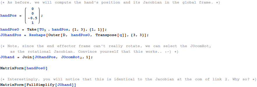
Let us start by computing the kinematics at the hand.
In[50]:=
Out[54]//MatrixForm=
![]()
Out[55]//MatrixForm=

Note, however, that the Jacobian has a clear null space along the rows corresponding to x and y rotations. As such, ![]() and
and ![]() are not controllable, and so we shall remove them from our Jacobian. In addition, given any three out of x, y, z, or
are not controllable, and so we shall remove them from our Jacobian. In addition, given any three out of x, y, z, or ![]() , we can also determine the fourth because the robot only has three degrees of freedom. We can thus only control z + two out of x, y, and
, we can also determine the fourth because the robot only has three degrees of freedom. We can thus only control z + two out of x, y, and ![]() .
.
In[56]:=
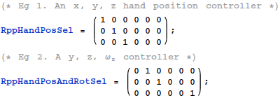
For the remaining tutorial, we shall pick the xyz position controller. You may experiment with the other one yourself.
In[58]:=
![]()
Out[59]//MatrixForm=
![]()
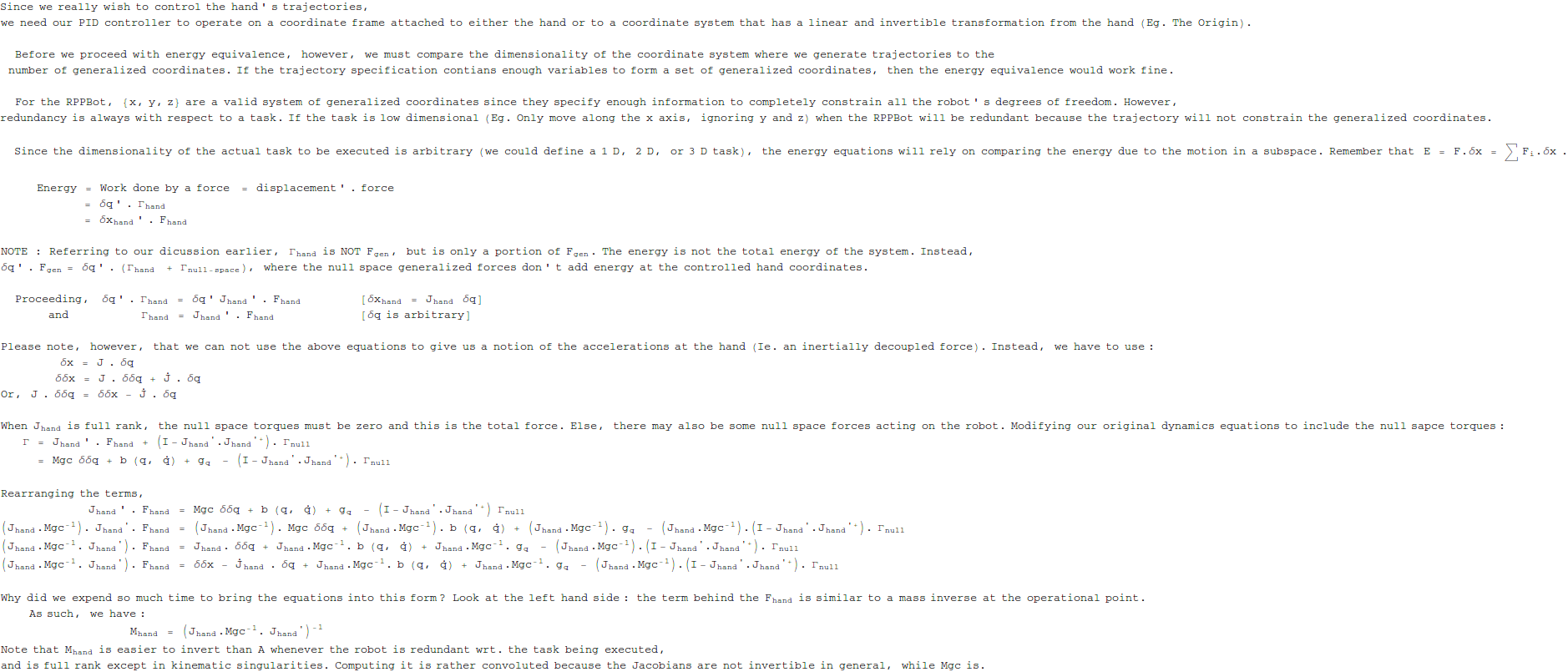
Energy Equivalence and Operational Dynamics : Hand
In[60]:=

Out[62]//MatrixForm=

Out[63]//MatrixForm=

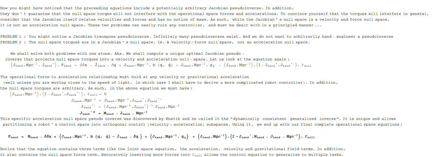
Reduced dynamic control equations in the operational coordinates
![]()
In[64]:=
![]()

In[65]:=
![]()
Out[66]//MatrixForm=
