Due August 5th, 11:59pm.
Written by Awni Hannun and Chris Piech.
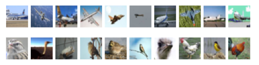
Figure 1: Various images of airplanes (top) and birds (bottom) from the CIFAR-10 dataset.
Introduction
In this assignment you are going to use computer vision to teach a program to classify images as either a bird or a plane with the help of the CIFAR-10 dataset.
In order to solve this problem, we will draw inspiration directly from the Primary Visual Cortex (V1) of the human brain. One commonly held hypothesis is that humans process natural stimuli such as images in V1 in multiple layers of representation, starting with the raw sensory stimulus and slowly building higher and higher levels of representation. For example in human vision the lateral geniculate nucleus (LGN) carries the raw sensory stimulus received in the retina to the first layer of V1. This first layer is hypothesized to have many neurons known as simple cells all of which code for different features in the input. In particular, much evidence points to these simple cells as being edge detectors, i.e. they each code for a specific edge of different orientation and translation within the image. The new representation of the input as the activations of these simple cells then becomes input to the next layer of V1 processing, which hopefully makes the task of understanding the input easier.
Not only will you learn a feature representation of images similar to the first layer of processing in V1, but you will do so with unsupervised learning. In other words, the algorithm isn't told via supervision or hardcoded in any other way to learn to represent an image as it's component edges. Amazingly, that's what it will find to be most important features in an image on its own!
In this assignment you will implement K-mean clustering to learn features from the raw input image pixels. These features will then give a higher level representation of the image which we can then feed to a classifier with the hope of making the classification task somewhat easier.
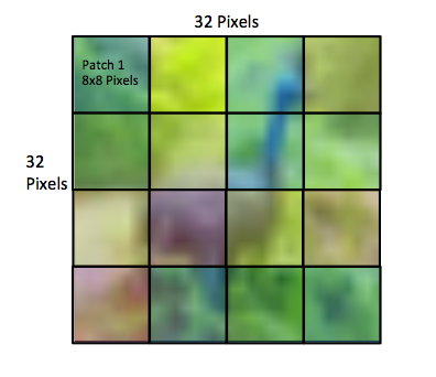
Figure 2: The sixteen patches of size 8x8 pixels corresponding to an image of size 32x32 pixels.
The full pipeline of the learning procedure will work as follows:
- Unsupervised Learning: Implement K-means to learn K centroids for image patches. These patches are small contiguous regions of the training set of images (Fig 2).
- Feature Extraction: Use the K centroids found in part 1 to extract features from each image. to feed into a supervised classifier. The feature extraction creates features for each patch of an image (Fig 2) using the K centroids from part 1. The full feature representation for an image is then the feature representations for all of its patches.
- Supervised Learning: Use the extracted features from part 2 in a logistic regression classifier. You'll use Maximum Likelihood Estimation (MLE) to learn the parameters of the classifier, which will be optimized with Batch Gradient Descent.
- Test: You will then evaluate performance of this classifier using a test set.
The code for this project contains the following files, available as a zip archive.
Key files to read:
featureLearner.py |
This file defines an object has methods that both run K-means unsupervised learning and feature extraction. You will modify this file in the assignment. Do not change existing function names, however feel free to define helper functions as needed. |
classifier.py
| This file defines an object for training and testing the logistic regression classifier. You will modify this file. Do not change existing function names, however feel free to define helper functions as needed. |
evaluator.py |
This file contains code to evaluate how your classifier performs on the test set. You should not need to modify this file but may want to read through the comments to understand how it works. |
util.py |
This file contains the Image class which will create objects that represent data for each image. Also contained in this file are several helper methods for viewing features and images. You should not need to modify this file although you should read through it to understand how it works. |
Submission: Submission is the same as with the Pacman and Driverless Car assignments. You will submit the files
featureLearner.py and
classifier.py. See submitting for more details.
Evaluation: Your code will be autograded for technical correctness. Please do not change the names of any provided functions or classes within the code, or you will wreak havoc on the autograder. However, the correctness of your implementation -- not the autograder's judgements -- will be the final judge of your score. If necessary, we will review and grade assignments individually to ensure that you receive due credit for your work.
Academic Dishonesty: We will be checking your code against other submissions in the class for logical redundancy (as usual). If you copy someone else's code and submit it with minor changes, we will know. These cheat detectors are quite hard to fool, so please don't try. We trust you all to submit your own work only; please don't let us down. If you do, we will pursue the strongest consequences available to us, as outlined by the honor code.
Getting Help: You are not alone! If you find yourself stuck on something, contact the course staff for help. Office hours and piazza are there for your support; please use them. We want these projects to be rewarding and instructional, not frustrating and demoralizing. But, we don't know when or how to help unless you ask.
Tasks
First, get familiar with the code. Load up the dataset and view a few images. Open the python interpreter (type python in the command-line) and run:
import util
train = util.loadTrainImages() # loads train as list of Image objects
train[0].view() # views first image
train[106].view() # views 106th image
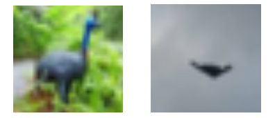
Figure 3: An example from each image class. Left: A bird, Right: A plane.
You should see the two images in Fig 3. In the training set planes are given the label 0 and birds the label 1. To see the label of an image type:
train[0].label # bird label
train[106].label # plane label
1. Unsupervised Learning
In this part of the task you will implement K-means clustering to learn centroids for image patches. Modify the file featureLearner.py and in this file the method runKmeans. When done with this part of the assignment you should be able to create a FeatureLearner object with centroids learned from your implementation of K-means.
Initialize K-means with random centroids drawn from a standard normal distribution.
In order to determine if K-means has converged, evaluate and print the residual sum of squares (RSS) after each iteration. RSS is defined as the sum of squared distances of each training patch to its closest centroid.
Where $m$ is the number of patches, $x^{(i)}$ is the $i$th patch and $\text{Centroid}(x^{(i)})$ is the centroid that the $i$th patch is assigned to after the most recent iteration.
Test the K-means code with the provided test utility in evaluator.py by running:
python evaluator.py -k -t
If you've passed the test above, try running your K-means method with a bigger dataset. After 50 iterations of K-means with the first 1000 training images and 25 centroids, our RSS is $\sim 807,189 $. You should be able to get the same results by running the evaluator and seeding the random number generator with the -f flag.
python evaluator.py -k -f
Another way to determine if your K-means algorithm is learning sensible features is to view the learned centroids using our provided utility function. To view the first 20 learned centroids, run
python evaluator.py -k -f -vYour centroids should look similar to Fig 4. Notice how the centroids resemble edges amazingly similar to the receptive fields that activate the simple cells found in V1.
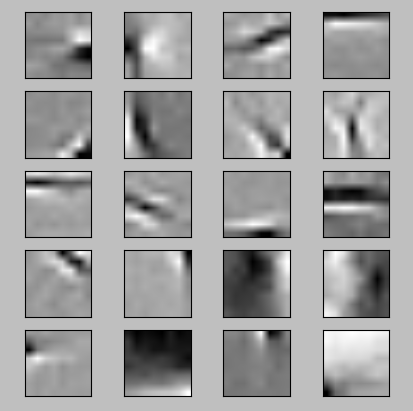
Figure 4: 20 centroids learned from K-means on patches from the first 1000 training images. Notice the edges!
Numpy: Some Numpy functions that may come in handy:
2. Feature Extraction
In this portion of the assignment you will implement the extractFeatures method in the featureLearner.py file. This method takes one image object at a time, gets the patches from that image object and then extracts features for each patch. Return the features in a form that will be useful in your supervised classifier. Each image will have $16$x$K$ features where $16$ is the number of patches per image and $K$ is the number of centroids learned in part 1. For each patch of the image, the feature values are the distance to the centroid if that distance is less than the average distance from that patch to all centroids and zero otherwise.
Where $f_{k}(x)$ is the $k$th feature for patch $x$, $\mu(x)$ is the average distance from $x$ all $K$ centroids and $c_k$ is the $k$th centroid.
Test your feature extraction code by running
python evaluator.py -e
3. Supervised Learning
In this part of the assignment you will implement a logistic regression classifier. First fill in the method train in the file classifier.py. In the train method, first learn the K-means centroids and extract features with the FeatureLearner object you built in parts 1 and 2. After that implement gradient descent to minimize the negative log-likelihood of the data. Initialize the parameter vector $\theta$ from a zero-mean gaussian with 1e-2 standard deviation ($\sim \mathcal{N}(0,1e-2)$).
You can test your logistic regression classifier by running
python evaluator.py -s
Also, while developing this part, to save time in computation you can run a toy version of the full pipeline by passing evaluator the -d flag.
python evaluator.py -d
Run gradient descent for self.maxIter=5000 iterations before stopping. After running gradient descent for 5000 iterations using only the first 1000 training images and a learning rate $\alpha=1e-5$, our negative log-likelihood evaluated to $823.6$.
Next implement the test method in the classifier.py file. This method takes as input a list of test Image objects and makes a prediction as to whether each image is a plane or a bird (0 or 1 respectively).
Now you are ready to run the entire pipeline and evaluate performance! Run the full pipeline with (include the -f flag to recreate our results):
python evaluator.py
The output of this should be two scores, the training and the testing accuracy. Following the steps above our classifier achieves 81.8% accuracy on the training set and 73.2% accuracy on the test set.
4. Extensions (Optional)
README file in your submission that documents everything you did. Some suggestions for extensions include:
- Get classification accuracy high! We will give bonus points to student with best classification accuracy. Note all extra work should be done outside of existing functions in order to not mess up the autograder. Report your best accuracy in your
README. We will run your code to verify this. - Try out using a different linear classifier, such as a linear SVM, and report how it performs.
- Overfit the training data with many centroids and add a regularizer to your cost function to see if you can improve generalization error
- Anything else you can dream up!
References
- Learning Feature Representations with K-means, Adam Coates and Andrew Y. Ng. In Neural Networks: Tricks of the Trade, Reloaded, Springer LNCS, 2012.(pdf)
- An Analysis of Single-Layer Networks in Unsupervised Feature Learning, Adam Coates, Honglak Lee, and Andrew Y. Ng. In AISTATS 14, 2011.(pdf)
- Learning Multiple Layers of Features from Tiny Images, Alex Krizhevsky, 2009. (pdf)
Project 3 is done!