
Overview
A significant amount of work has been done on scalable video coding to deal with the heterogeneous condition over the Internet. However, scalable coding is only part of the problem and it should be appropriately used at transmission time. One router mechanism that limits the effect of loss to those parts of a stream that contribute least to quality, is priority dropping which is provided by the AF class of the DiffServ standards. In this project, we first show the merit of combining scalable encoding with priority dropping in terms of multiplexing gain, gradeful quality degradation over a wide range of network loss rates, and ability to handle short-term congestion. In the second part of the project, we provide some guidelines on how to configure parameters of both layering scheme and priority dropping in the scenario of video traffic over a single hop.
Keywords
Video Transmission, H.263+, SNR scalability, Priority Dropping, Differentiated Services networks.Table of Contents
1. Introduction
2. Background
3. Simulation Setup
4. Results and Discussion
5. Conclusions and Future Work
6. References
Today's Internet is composed of heterogeneous computing machines and it only delivers data on a best-effort basis. To address the issue of streaming video distribution over the Internet, infrastructure-oriented people advocate faster routing/switching engines and the support of Quality of Service(QoS) in the network nodes. Taking a complementary approach, application-oriented people try to find innovative streaming techniques to adapt to the current Internet environment and to fully utilize their fair share of network resources.
Actual video transmission over the Internet uses network mechanisms to appropriately handle scalable video. One way to provide different levels of QoS to different layers of a video stream is priority dropping. This project is devoted to the question of drop priority for the transmission of scalable video in contexts where packet drops, rather than packet delays, are the primary determinant of application performance.
Our project is motivated by [4] and follows steps to show that priority dropping provides graceful degradation of quality over a wide range of network loss rates and demonstrate the multiplexing gain of supporting more streams with the same perceived quality. It differs from [4] in that (i) we use H.263+ video streams as opposed to MPEG-2 (ii) we focus on SNR scalability rather than on data partitioning that exists only in MPEG-2 (iii) we study real buffer loss rather than uniform artificially applied loss (iv) we try to compare and see how feedback and priority dropping mechanisms fit in the picture of video transmission (v) we try to provide guidelines for configuring both the layering and buffer management parameters.
In the next section we provide background on scalable video coding and transmission over the packet-based network.In Section 3 we describe the simulation setup for our transmission system. In Section 4 we present our results concerning the benefits of combining priority dropping and layered video in terms of multiplexing gain, graceful quality degradation over a wide range of loss rates, and ability to handle short-term congestion. In the same section, we also provide some guidelines for configuring buffer management and layering parameters. We conclude and outline future work in Section 5.
The scalable video coder produces a bit stream, decodable in multiple layers, which provides different levels of quality. It allows computation-time and memory-limited decoding on less powerful hardware platforms, and it can substantially improve the quality of video transmitted over error-prone channels such as the Internet or wireless. Temporal, SNR, and spatial scalability have been defined in the international video coding standards, e.g., the H.263 [9]. All of these types of scalable video consist of a base layer (BL) and one or more enhancement layers (ELs), according to their contribution to quality.
In this project, we focus on the SNR scalability. Because compression introduces artifacts and distortions, the difference between a reconstructed picture and its original in the encoder is a nonzero-valued picture, a so-called coding error. With SNR scalability, these error pictures are encoded and sent to the decoder, producing an enhancement to the decoded picture. The extra data serves to increase the signal-to-noise ratio of the video picture, hence the term SNR scalability. Figure 1 shows the temporal dependency as well as the dependency between BL and EL.
Figure 1: SNR Scalability
![]()
Figure 2: Transmission over the Internet
The transmission of high quality video over the Internet faces many challenges. Fortunately enough, different parts of an encoded stream contribute unequally to the quality. This property can be exploited at transmission if network mechanisms use the available bandwidth to transit the most important parts of the stream, thus maximizing the perceived quality. Let us examine such mechanisms.
First of all, the Internet is a heterogeneous environment and many links experience high loss which leads to significant quality degradation of a single video stream. Note that, as also shown in this project, even small loss rates may result in significant quality degradation due to the temporal dependencies in the encoded bitstream. To limit that degradation, the idea of dynamically adapting the encoding parameters at the source based on feedback has been considered. A source might alternatively react to congestion by dropping or adding a layer. However, adaptation at the source cannot always overcome the large variations in packet loss and is limited by the delay in the feedback and the accuracy in estimating the bottleneck bandwidth.
Second, the loss experienced due to congestion episodes in the Internet varies over time due to both the variability of the aggregate load and the variability of individual flows/streams . Even if video traffic is separated from the bursty data into a different queue, loss may still occur due to the variability of the video streams themselves. Limiting the variability in the aggregate load is a matter of proper admission control. Limiting the variability of individual video streams or TCP flows is a matter of smoothing/shaping. However, such an approach, is complicated and has not be successful so far in the Internet, thus the failure of Integrated Services.
Another challenge is the heterogeneity of the receivers in terms of processing capabilities and receiving bandwidths. This problem is best addressed by scalable encoding. McCanne et.al. proposed in [5] that, in the multicast receivers adapt to congestion by subscribing/unsubscribing to layers multicast by the source. However, this approach does not have fine bandwidth granularity and is limited by the round trip time from the source to the receivers.
The focus of our project is on priority dropping, another mechanism that can protect the most important parts of a stream during network congestion. Priority Dropping can detect congestion where and when it happens and can limit its effect by intelligently dropping the data with the least effect on perceived quality. However, one might still want to use source and/or receiver driven adaptation, to handle congestion over longer times scales and prevent waste of network resources from the source until the congested router.
Priority dropping will be made possible in the Internet by means of the Differentiated Services architecture (DiffServ) currently under standardization by the IETF. In this architecture, packets are marked as belonging to a few aggregates and are treated by routers according to this marking. The strong point of this architecture is its scalability, as routers need to keep state only per few aggregates as opposed to all flows. The structure of a typical DiffServ node is shown in Figure 3.
Figure 3: Example of a DiffServ Node
The element of interest to us is the so-called Assured Forwarding (AF) Per Hop Behavior because it implements the priority dropping mechanism. The standards define four AF classes. Each Af class has a minimum bandwidth guarantee and can differentiate among 3 different levels of drop precedence. The definition [2] does not require but does imply that each AF class should use a separate queue. Figure 14 shows a queue with 2 levels of drop precedence.
The DiffServ architecture does not dictate the kind of traffic aggregate that should use an AF queue. Whether or not Video should be mixed with or separated from dissimilar traffic types, is by itself the topic of another project. In the scope of our project, we consider an AF queue used exclusively by video traffic. Fortunately, there is enough evidence in the literature [3] that this is a good design choice.
The performance of a video transmission system is significantly influenced by various implementation issues like packetization and error concealment. Our system is shown in Figure 4 and each component is explained in detail.
Figure 4: System Block Diagram
The main and interfering sequences were packetized following the payload format specified in RFC 2429: RTP Payload Format for H.263+ Video Stream [8]. In our simulation, the packet size is set to 1500B (MTU) from which 20B consist the IP header, 8B the UDP header, 12B the RTP header, as shown in Figure 5.

Figure 5: RTP Payload Format
The payload of the packet is set to 1456 bytes with the shortest H.263 header of 4 bytes, which corresponds to mode A supporting fragmentation at frame boundaries. Because we used low frame rates and large packet sizes, it turned out that small (P) frames could fit in a single packets while some I frames use 1-2 packets. However, no frames from different layers are ever put into the same packet.The packets of each packetized video stream are then marked with one of two markings: packets of the base/enhancement layer are marked with low/high drop precedence respectively. In scenarios with non layered sequences, there was no reason to mark.
The main and the background streams were then multiplexed over a single 1.5 Mbps link. The buffer size was 100KB, i.e. 67x1500B packets. In the experiments with nonlayered streams, the buffer management was considered to be DropTail. In the experiment with layered streams, the buffer management was considered to implement priority dropping with 2 drop precedences and parameters specific to each experiment.
We used the Network Simulator [10] to simulate the "network". Although for this project we considered only a single link, NS enables us to easily extend our work over complex topologies. We had to convert the video traces into the NS format, implement the priority dropping[11], collect and parse the results in order to inform the receiver which packets of the main video stream are lost in the buffer.
Packet loss itself is not a good measure of quality degradation. Instead, we evaluate the goodness of the pictures on the basis of the peak signal- to-noise ratio (PSNR) of the resulting frame difference between the original sequence and the decoded, defined by
![]()
We use the average PSNR as our main performance measure. When the typical frame freeze is applied due to the packet loss in our simulation, we also use the PSNR of the frozen frame for the lost frames. However, as shown in Figure 6, averaging over time hides the number of frame freezes and makes some comparisons unfair. Therefore, subjective quality perceived by the end users should be considered in the future to determine whether these applications are adopted [7].
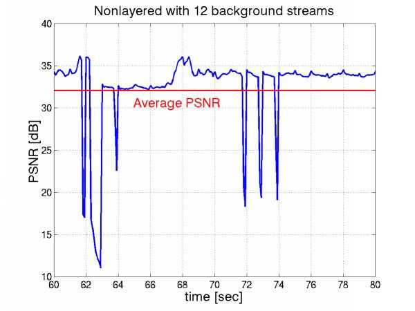
Figure 6: PSNR Varying over Time
In this section we present and discuss our simulation results.
Simulation setup: Let us consider the foreman sequence multiplexed with 10-20 streams over a single 1.5Mbps link. We vary the number of MUX streams and we measure the PSNR for the foreman sequence. Each layered stream has a base layer of 50kbps and an enhancement layer of 86kbps, while each nonlayered stream has 128 Kbps rate. The buffer size is 100KB (or 67x1500B), instantaneous queue size is used and dropping curve(s) have 90 degrees angle.. First we do the experiment with a DropTail queue and nonlayered sequences. Then we use layered sequences and 2 drop precedences with thresholds 40 and 66 packets.
Figure 7: Multiplexing Gain
Figure 7 shows the average PSNR of the Foreman sequence vs the number of streams multiplexed over the link. We see that the PSNR is almost constant if the streams are layered and the priority dropping is used while it drops drastically if they are not layered. The overhead for the non layered streams is negligible. In other words, we can support almost double number of streams meeting the same PSNR for our target sequence, if we use layered streams together with priority dropping.However, note that this is the average PSNR. What actually happens in the nonlayered case is that the quality of individual frames is high but there are many freezes.
In this section we consider that the Foreman sequence experiences some loss and present the perceived quality after error concealment in Figure 8. The X-axis is the average rate of the received sequence (considering only payload without headers). Decreasing received bitrate can equivalently be thought as increasing loss rate. The Y-axis is the average PSNR of the received and concealed Foreman sequence.
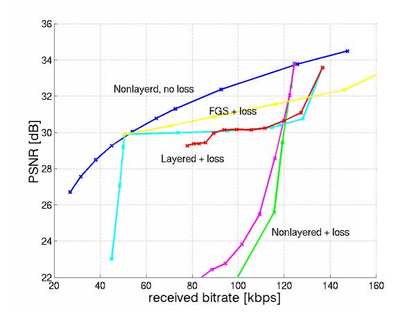
Figure 8: Graceful Degradation with Loss
Let us now discuss in detail these curves.
Our targeting quality without loss is around 34 dB which can be achieved by the nonlayered sequence at 128kbps. The same quality can be obtained by layered sequence at the cost of overhead. The target bitrate is 56 kbps for BL and 136kbps in total.
However in practice, when the NL stream is transmitted over a network it will experience some loss. We apply uniform loss on the sequence and we notice that by applying uniform loss from 128kbps to 100kbps, the quality drops drastically from 34dB to 22dB. In practice the loss experienced will not be uniform across the sequence but it will be buffer loss. We find the average loss rate experienced by Foreman due to its multiplexing with the other video streams,as in Figure 7, and we plot the corresponding average PSNR. The curve we get for the video buffer loss is very close to the uniform loss curve and actually it is slightly better. We believe that buffer bursty loss works better with our error concealment, as we explain later.
Then, we look at the layered Foreman sequence. If the entire base and enhancement layer is correctly received, it will have on average a total rate of BL+EL=136kbps. However, in practice, the stream will experience some loss over the network. First, we apply larger and larger uniform loss on the enhancement layer only and we see that the quality degrades gracefully until the entire enhancement layer is lost. As the base layer starts getting dropped, the quality drops drastically again. Then, we plot the rate of the Foreman sequence experiencing the same loss rate on average, but this time the loss is due to the multiplexing over the buffer in Figure 7. We get a curve very close to the one corresponding to the uniform loss. This is a very satisfactory observation because it verifies that the priority dropping handles the loss indeed intelligently by allowing it to affect only the enhancement layer. Another observation that one can make is that the quality of the layered video drops drastically at the first kbps of loss and then it remains almost constant. This is largely because of our concealment method that freezes at the last received frame. Therefore, losing a single EP frame is equivalent to losing all the EP frames until the next EI. We expect that if we used a packetization at GOB boundaries, we would get better error concealment and more graceful quality degradation. However, packetization at GOB level, does not make sense at the low rates of our sequences and for 1500B packets.
Indeed, when we try FGS, which does not have temporal dependency in EL, with buffer loss, we got much more graceful degradation at the cost of coding overhead as seen in Figure 8.
The most important observation to make on this figure, is the graceful degradation of quality of the layered sequence using priority dropping over a large bandwidth range [50,136kbps or 160kbps], compared to the drastic degradation of the layered sequence in the much more narrow bandwidth range [100,128kbps].
We think of priority dropping as a way of handling a limited variability in network bandwidth by protecting the base layer from loss.
Although priority dropping is one of the ways the network might handle scalable video, it is not the only one, as discussed in the "Transmission of Video" section. Feedback to the source might be useful. Here we consider a simple comparison among a feedback+reaction scheme and priority dropping in terms of their successful handling of the same congestion episode.
Let us consider a stream consisting of base (BL) and enhancement layer (EL) and a congestion episode for a period of time. The feedback+reaction scheme, Figure 9, is dealing with the congestion by dropping the EL after delay D and then adding EL again, with delay D after the episode finishes. Such a reaction is limited by the delay D and by the granularity of the EL, R. Priority dropping on the other hand, reacts to congestion immediately and by the appropriate rate reduction R(t)in the EL, as shown in Figure 10
Figure 9: Feedback and Reaction to Congestion
Figure 10: Priority Dropping Handling Congestion
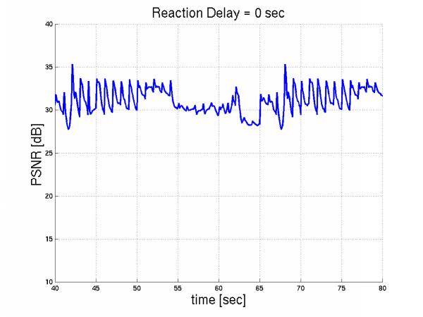
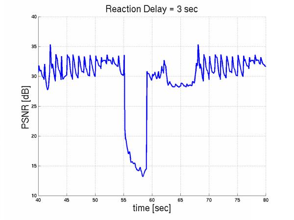
More specifically, let us considered 10 layered streams multiplexed over the 1.5Mbps link and 5 more interfering during the interval [55sec, 65sec].The initial streams react to this congestion by dropping their enhancement layer in [55sec+D, 65sec+D]. Here are the PSNR of the Foreman sequence over time for increasing reaction time.
The smaller the D, the better such a feedback scheme performs, in terms of avergae PSNR, as shown in Figure 11.
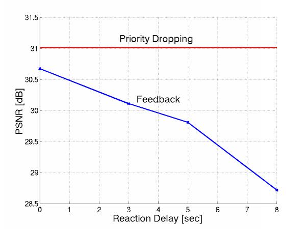
Figure 11: PD vs. Feedback
Priority dropping, reacts immediately, as shown in Figure 12.
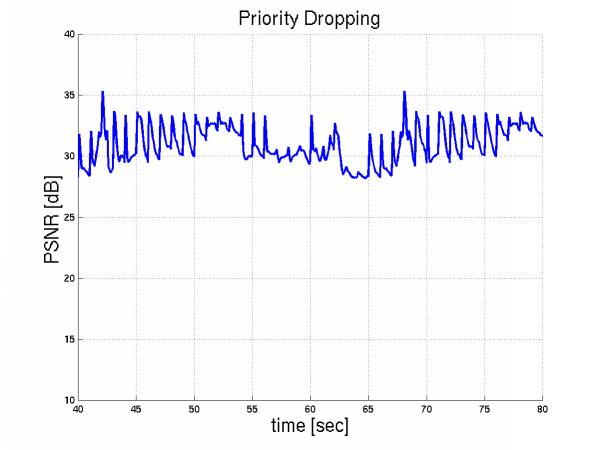
Figure 12: PD handling congestion
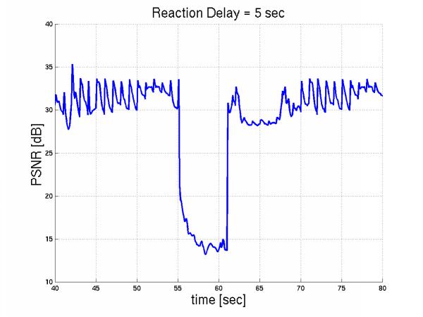
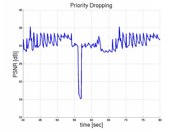
Then we applied even heavier congestion by introducing 10 additional video flows during the period [55,65sec] and we notice that congestion remains even if all initial streams backoff immediately. Priority dropping on the other hand, handled this episode more gracefully. Here is the foreman PSNR over time with reaction delay 5 sec and here is with priority dropping.
However, we realized that this was not a fair comparison between feedback schemes and priority dropping because we did not allow the source to adjust its base layer encoding parameters. Under the experiment we did, feedback could at best perform like priority dropping as shown in Figure 11. Therefore more work needs to be done to investigate this aspect.
We expect that priority dropping will prove to gracefully handle short term congestion and feedback to match the transmission rate to the bottleneck bandwidth and save network resources until the congestion point. Let us look at Figure 13. If we transmit a layered stream with BL at R2 and the total rate R, the priority dropping gracefully handles the loss from 0 upto R-R2, similarly to Figure 8. The loss beyond R-R2 will cause dropping of BL and thus, priority dropping cannot prevent quality degradation anymore. Then, feedback to the source to adjust the BL at R1 is a better solution.
Figure 13: How to handle congestion
Once the merit of using priority dropping for the transmission of layered video is established, the next question is how to tune the various parameters concerning both buffer management and layering.
An AF queue, with 2 drop precedences is shown in Figure 14. Base and enhancement layer packets are marked as low and high drop precedence respectively. Packets of each drop precedence are dropped according to a different dropping curve. Differentiation results from the fact that (i) high drop precedence packets start to get dropped earlier and (ii) they consider buffer occupancy to be the total number of packets in the queue as opposed to the lower drop precedence that consider buffer occupancy to be their own number only.

Figure 14: an AF queue with 2 drop precedences
So, what are the choices and the configurable parameters in such a queue?
First, one has to decide on the shape of the dropping curves . Should there be a slope indicating early drop (left curve: L_min < L_max ) or should there be a 90 degrees slope (right curve: H_min = H_max = H )? Our results indicate that early drop performs bad under all configurations, which makes sense because early drop was meant to signal adaptive TCP traffic and not UDP (video) traffic.
Second, one has to define what buffer occupancy in the X-axis of Figure 14. means. In RED-like buffer management, a moving average of the queue size is used to indicate the buffer occupancy as opposed to the instantaneous queue size. In our simulations, use of the instantaneous queue size performed always better.
The buffer occupancy for the BL packets means the number of BL packets in the queue. However, the buffer occupancy for the EL packets may mean either the number of EL packets in the queue or the total number including BL packets. We observed that the first, led to better perceived quality provided that the buffer thresholds were appropriately tuned. All the simulations shown in the web report, are performed with the latter option. The low drop precedence curve should consider low drop precedence packets only.
Figures 15 and 16 compare a RED-like buffer management (early drop & average queue size) and DropTail buffer management (90 degrees dropping slopes & use of instantaneous queue size) and show that RED-like leads to worse perceived quality, under all loads, Figure 15, and for all possible thresholds, Figure 16.
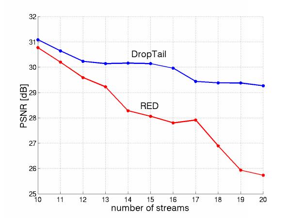
Figure 15: RED-like worse for all loads |
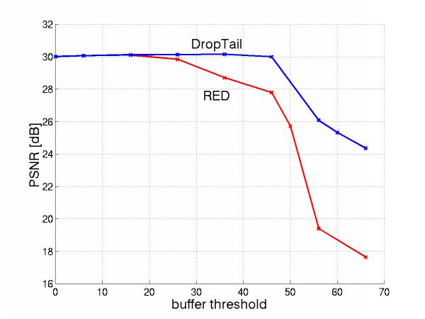
Figure 16: RED-like worse for all thresholds L: 0 < L < H |
Having shown the need to avoid RED-like mechanisms, the last question to ask concerning the configuration of the AF queue, is what are the appropriate thresholds L,H . By assigning the buffer thresholds L, H , we control how the buffer is distributed among base and enhancement layers. Let us fix H to Queuesize = 67 packets and vary the threshold for the enhancement layer. Figures 17 and 18 show the buffer occupancy across time for L=56 and L=16 respectively. Notice that in the case of L= 56, which almost equals to 66, there is still differentiation because the EL considers "occupancy" to be the number of both BL and EL in the queue.

Figure 17: Queue occupancy for base and enhancement for L=16 |
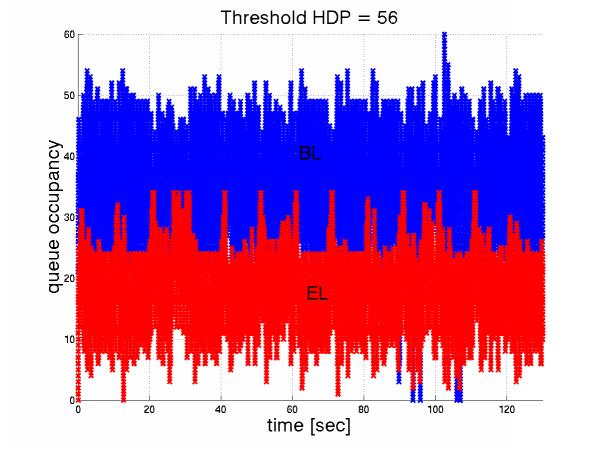
Figure 18: Queue occupancy for base and enhancement for L=56 |
By increasing L, we allow more EL packets in the queue and thus we decrease the loss in EL and increase it in BL, as shown in Figure 19.
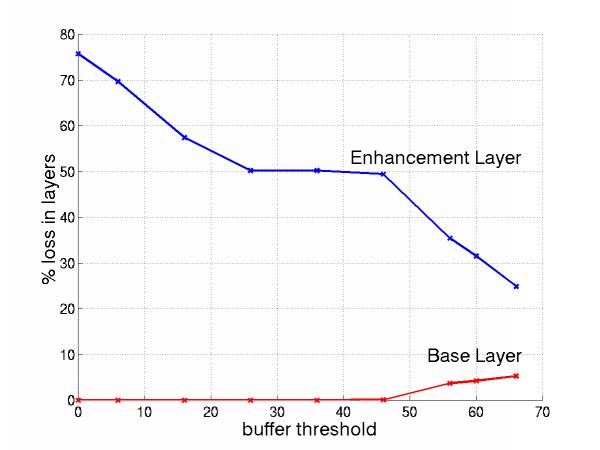
Figure 19: Loss in Layers
Therefore, by changing L we affect the PSNR. Fortunately enough, we notice that PSNR is NOT sensitive to the exact value of threshold L for a wide range of values. Figure 16 (RED) shows this lack of sensitivity to the choice of L for RED and non RED and Figure 21 (BL) shows the lack of sensitivity to the choice L, for different base layers.
Another quesiton is how to choose the rates of each layer. For the experiments of this section we use 3 different base layers for the Foreman sequence and the same target (BL+EL) quality.
Figure 20, shows how avg PSNR of Foreman degrades when the loss increases by adding more streams. The thiner the base layer the lower the PSNR at low loads/loss rates but the more constant the quality across a wide range of loss. We see that the curve for large BL (64kbps) degrades drastically early, when its base layer starts getting dropped. Figure 21, shows again practically lack of sensitivity to the specific value of buffer threshold for all base layers.
We are thinking of base layer as the amount of data that should absolutely be shielded by loss. The larger the bandwidth variations expected, the more consevative the choice of the base layer should be. Therefore the base layer should be chosen having in mind the bandwidth capabilities of the target clients (similarly to the way RealNetworks do with their SureStreams) and the variations in the bottleneck bandwidth. Thus, the base layer should be chosen slightly below the poorest receiver bandwidth. The next enhancement layer should be the difference of bandwidthes of the 2 poorest receivers and so on. Receivers should subscribe to the appropriate amount of layers, according to their capabilities. Priority Dropping would take care of short term congestion. This is all consistent with Figure 13.

Figure 20: Quality with different BL rate for all loads |

Figure 21: Quality with different BL rate for all thresholds |
In this project, we studied the benefits of using priority dropping in routers to handle layered video. We also gave some guidelines for configuring such a system.
The most important observations from multiplexing streams over a single hop are the following:
The most important observations from the experiments concerning the configuration of the AF queue are that:
The most important observations concerning the choice of base layers are the following:
We believe that the problem we studied in this project is a meaningful and rich research problem. We only addressed some of its aspects and we would like to follow up on it. Some improvements together with some brand new experiments would support and extend our current work.